AI Engine DevelopmentSee Vitis™ Development Environment on xilinx.com See Vitis-AI™ Development Environment on xilinx.com |
Single-Kernel FIR Filter Implementation
In this first part of the tutorial you will use a basic filtering application and analyze the performance that can be achieved.
Navigate to the SingleKernel directory to continue.
Filter Description
Thoughout this tutorial you will use and reuse the same filter with complex coefficients. This filter has 32 coefficients (or taps) and has no symmetry characteristics.
{   -82,  -253},{     0,  -204},{    11,   -35},{  -198,   273},
{  -642,   467},{ -1026,   333},{  -927,     0},{  -226,   -73},
{   643,   467},{   984,  1355},{   550,  1691},{     0,   647},
{   538, -1656},{  2860, -3936},{  6313, -4587},{  9113, -2961},
{  9582,     0},{  7421,  2411},{  3936,  2860},{  1023,  1409},
{  -200,  -615},{     0, -1778},{   517, -1592},{   467,  -643},
{  -192,   140},{  -882,   287},{ -1079,     0},{  -755,  -245},
{  -273,  -198},{    22,    30},{    63,   194},{     0,   266}
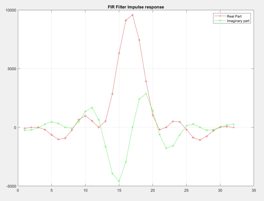
The output of this filter will have a much higher amplitude than the input. A scaling factor of 2^15 should be applied to get back to normalized data. On debugging phase, when only impulses are given to the filter, the scaling factor can be reduced to 1 so that we can verify that the output looks like the impulse response of the filter.
Designing the Kernel
Before building a kernel to implement FIR filtering, consider the following:
What kind of interface will I use?
How many coefficients do I have?
How will it influence the size of the data register and coefficient register?
How many lanes can I use in my intrinsics?
When will I schedule data reading and writing?
Interfaces
There are two types of interfaces: windows and streams. The bandwidth of the memory (where windows are stored) access is much higher than the streams: 2x32 GB/s vs. 2x4 GB/s. Even if the memory bandwidth from the processor is very high, they must be filled in either by another AI Engine (bandwidth 32 GB/s) or streams (2x4GB/s). Either way, somewhere in the cascade of kernels the origin of the data will be outside of the AI Engine array (PL, DDR, …) implying a stream source.
Window interfaces are used in a ‘ping-pong’ manner to allow for continuous data transfer while maintaining continuous processing. When multiple kernels are mapped to the same AI Engine and they communicate through windows, these windows use a single buffer because the kernels do not run at the same time. Ping-pong buffering means that the data are processed only when the buffer is completely filled in, incurring a minimum latency of the duration of this buffer filling. When an AI Engine kernel uses window interfaces, it must acquire a lock to gain access ownership to this memory. Lock acquisition and release takes a minimum of seven cycles per lock, which reduces the time allowed for processing.
As a rule of thumb, 750 Msps is the maximum sample rate for which window interfaces are a viable solution. When the kernel processing duration is just a fraction of the time it takes to fill in the input window, this is reflected by a utilization ratio much below 1 and multiple kernels can be mapped onto a single AI Engine.
In this tutorial, the goal is to achieve the maximum performance filter implementation, leading to a streaming interface at the input and the output.
Data and Coefficients Management
The data register is limited to 1024 bits (v32cint16) and the coefficient register maximum bitwidth is 512 bits (v16cint16). Having a streaming interface (single stream to start with), four cint16 can be read in one instruction, but it takes four clock cycles to be able to perform the same operation again. Reading four samples at a time allows the use of mul4 and mac4 intrinsics.
Not all intrinics exist for the AI Engine. Only two intrinsics will handle four lanes for complex 16 bits x complex 16 bits:
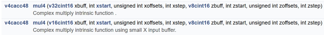
In this tutorial finite length loops (by default 512 input/ouput samples) are assumed for ease of debugging. This number of iterations can be increased as desired up to infinite loops (while(1) { ...}). Between two calls of the kernel, the status of the delay-line of the filter needs to be maintained. This delay-line must be at least 31 samples for a 32-tap filter. 32 samples fit in a Y register that’s why we will use a v32cint16 variable to keep this delay-line. At the beginning of the kernel call this delay-line will be loaded from the memory, and at the end it will be stored there. For the coefficients there is no option: it will be v8cint16.
A mul4 operating on cint16 x cint16 can perform eight operations in one clock cycle, leading to two operations per lane.
Coefficients and Data Update Scheduling
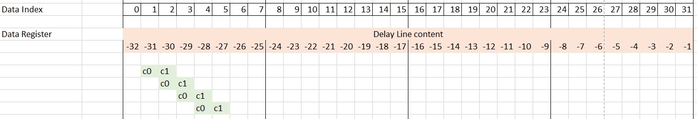
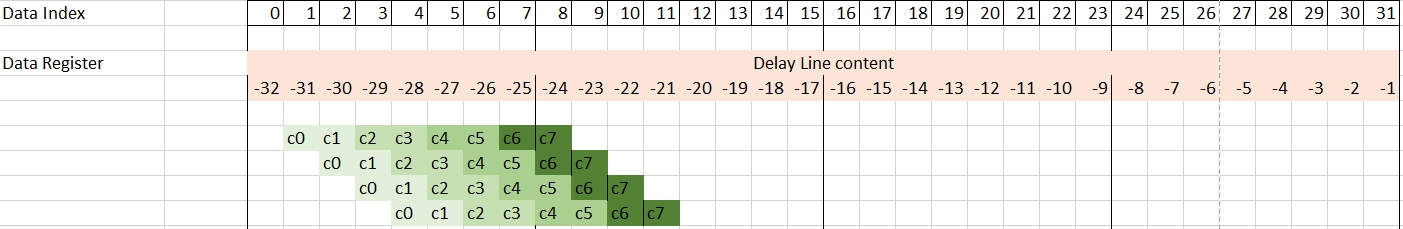
Before the first iteration the delay-line, the status is read to update the Y register. It will contain all the necessary previous data: { d(-32), d(-31), ... , d(-2), d(-1)}. The first output will be the result of the following operation:
y(0) = d(-31).c(0) + d(-30).c(1) + ... + d(-1).c(30) + d(0).c(31)
where the array c is the array of coefficients. Use a table to organize operations scheduling (excel for example):
This image represents the following equation:
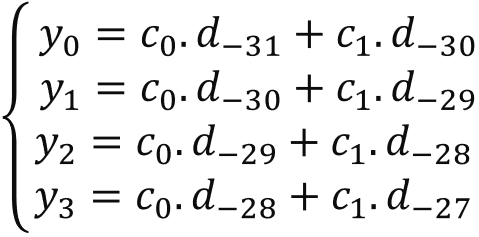
Following this first mul4 operation 15 mac4 operations should be used to finih the computation of {y(0), y(1), y(2), y(3)}.
Use darker and darker green to represent the next three mac4 operations
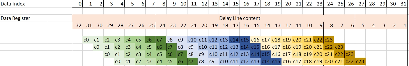
With these operations performed, the eight coefficients that were in the the v8cint16 have been used, and it is time to update them. These operations should be followed by eight mac4 operations:
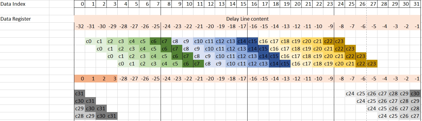
The next block of four mac4 operations will wrap around and reuse the begining of the data register. It is time to load four new samples from the stream and finish the operations:
Now that the computation of {y(0), y(1), y(2), y(3)} has been completed, the next four outputs {y(4), y(5), y(6), y(7)} have to be computed. As can be seen in the previous image, the next computation must start with index 5 in the data register. As in the previous set of output samples, the data register will be updated just before the group of four mac4:
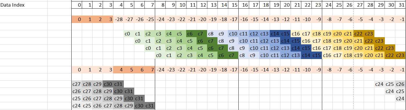
In order to have a regular inner loop, 32 output samples (eight groups of four) will be computed in the inner loop.
Now take a look at the related C code to implement all these operations. The program takes advantage of the templatization of the function and of the inclusion of the state in the class itself:
namespace SingleStream {

template<int NSamples,int ShiftAcc>
class FIR_SingleStream {
private:
	alignas(32) cint16 weights[32];
	alignas(32) cint16 delay_line[32];

public:
	FIR_SingleStream(const cint16 (&taps)[32])
	{
		for(int i=0;i<32;i++)
		{
			weights[i] = taps[i];
			delay_line[i] = (cint16){0,0};
		}
	};

	void filter(input_stream_cint16*  sin,output_stream_cint16*  sout);

	static void registerKernelClass()
	{
		REGISTER_FUNCTION(FIR_SingleStream::filter);
	};
};

}
The taps will be provided during instantiation of the class. The constructor initializes the internal array and sets the delay line to zero. In the template, two arguments define the number of iterations of the inner loop and the shifting value that will be applied to the accumulator before sending the calculated y-values to the output stream.
Function, declaration, and variable initialization are as follows:
template <int NSamples,int ShiftAcc>
void FIR_SingleStream<NSamples,ShiftAcc>::filter(input_stream_cint16* sin,output_stream_cint16* sout)
{
	v8cint16 *coeff =  (v8cint16*) weights;
	v8cint16 taps = undef_v8cint16();
	v32cint16 *ptr_delay_line = (v32cint16 *)delay_line;
	v32cint16 data = *ptr_delay_line;

	v4cacc48 acc = undef_v4cacc48();
    ...
The function filter has two stream arguments: sin and sout for stream-in and stream-out. The pointers to the coefficients and the data are prepared so that they can be loaded using pointer addressing.
// Computes 32 samples per iteration
	for(int i=0;i<NSamples/32;i++)
		chess_prepare_for_pipelining
		chess_loop_range(NSamples/32,NSamples/32)
	{
        taps =  *coeff++;   // Get the coefficients for the Green block
        acc = mul4(data,1,0x3210,1,taps,0,0x0000,1);
        acc = mac4(acc,data,3+2,0x3210,1,taps,2,0x0000,1);
        acc = mac4(acc,data,5,0x3210,1,taps,4,0x0000,1);
        acc = mac4(acc,data,7,0x3210,1,taps,6,0x0000,1);

        taps =  *coeff++;   // get the coefficients for the Blue block
        acc = mac4(acc,data,9,0x3210,1,taps,0,0x0000,1);
        acc = mac4(acc,data,11,0x3210,1,taps,2,0x0000,1);
        acc = mac4(acc,data,13,0x3210,1,taps,4,0x0000,1);
        acc = mac4(acc,data,15,0x3210,1,taps,6,0x0000,1);

        taps =  *coeff++;   // Get the coefficients for the yellow-brown block
        acc = mac4(acc,data,17,0x3210,1,taps,0,0x0000,1);
        acc = mac4(acc,data,19,0x3210,1,taps,2,0x0000,1);
        acc = mac4(acc,data,21,0x3210,1,taps,4,0x0000,1);
        acc = mac4(acc,data,23,0x3210,1,taps,6,0x0000,1);

        data = upd_v(data,0,readincr_v4(sin));  // Update the data register

        taps =  *coeff++;   // Get the coefficients for the Grey block
        acc = mac4(acc,data,25,0x3210,1,taps,0,0x0000,1);
        acc = mac4(acc,data,27,0x3210,1,taps,2,0x0000,1);
        acc = mac4(acc,data,29,0x3210,1,taps,4,0x0000,1);
        acc = mac4(acc,data,31,0x3210,1,taps,6,0x0000,1);

        writeincr_v4(sout,srs(acc,ShiftAcc)); // Write on the output stream
        coeff -= 4;     // Realign the coefficients pointer
        ...
These four blocks have to be written eight times with different parameters to compute the 32 output samples. In the code that is published, two macros are defined to make this exercise a little easier:
#define MULMAC(N) \
		taps =  *coeff++; \
		acc = mul4(data,N,0x3210,1,taps,0,0x0000,1); \
		acc = mac4(acc,data,N+2,0x3210,1,taps,2,0x0000,1);\
		acc = mac4(acc,data,N+4,0x3210,1,taps,4,0x0000,1);\
		acc = mac4(acc,data,N+6,0x3210,1,taps,6,0x0000,1)

#define MACMAC(N) \
		taps =  *coeff++; \
		acc = mac4(acc,data,N,0x3210,1,taps,0,0x0000,1); \
		acc = mac4(acc,data,N+2,0x3210,1,taps,2,0x0000,1);\
		acc = mac4(acc,data,N+4,0x3210,1,taps,4,0x0000,1);\
		acc = mac4(acc,data,N+6,0x3210,1,taps,6,0x0000,1)
Compilation and Analysis
Ensure that the InitPythonPath has been sourced in the Utils directory.
Navigate to the SingleKernel directory. In the Makefile, three methods are defined:
aieCompiles the graph and the kernels
aiesimRuns the AI Engine System C simulator
aievizRuns
vitis_analyzeron the output summary
Have a look at the source code (kernel and graph) to familiarize yourself with the C++ instanciation of kernels. In graph.cpp the PL AI Engine connections are declared using 64-bit interfaces running at 500 MHz, allowing for maximum bandwidth on the AI Engine array AXI-Stream network.
To have the simulation running, input data must be generated. Change directory to data and type GenerateStreams. The following parameter should be set for this example:
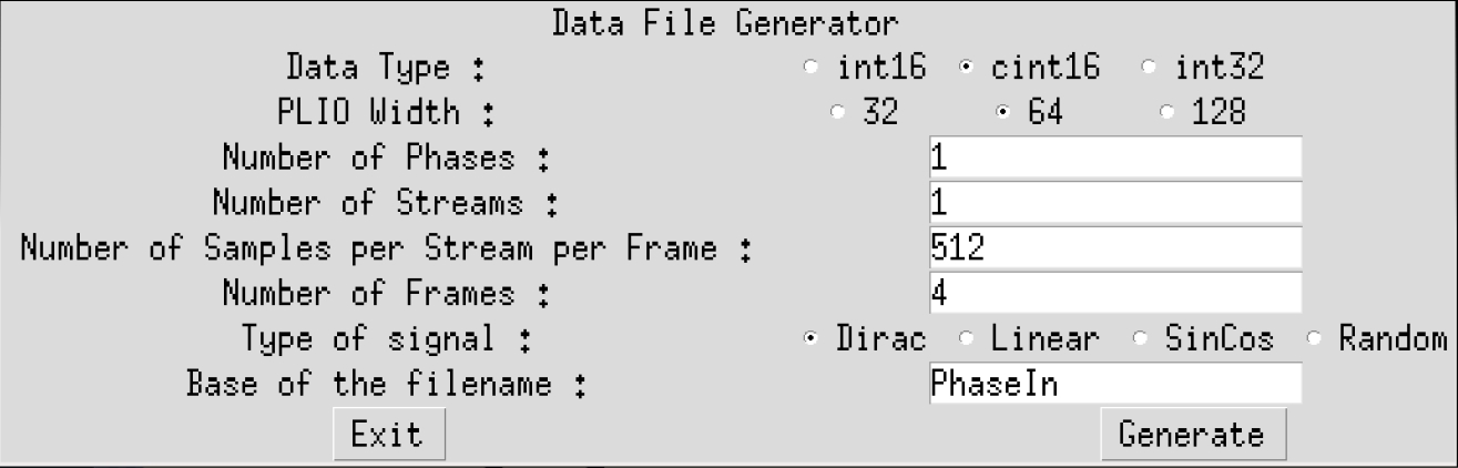
Click on Generate then on Exit. The generated file PhaseIn_0.txt should contain mainly 0’s, with a few 1’s and 10’s.
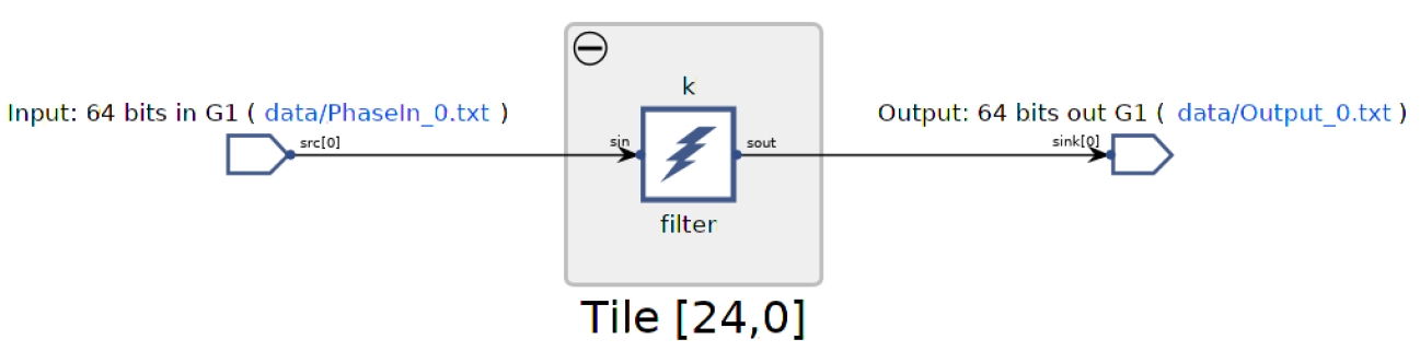
Type make all and wait for vitis_analyzer GUI to display. The Vitis analyzer is able to show the graph, how it has been implemented in the device, and the complete timeline of the simulation. In this specific case the graph is very simple (a single kernel) and the implementation is on a single AI Engine.
Click Graph to visualize the graph of the application:
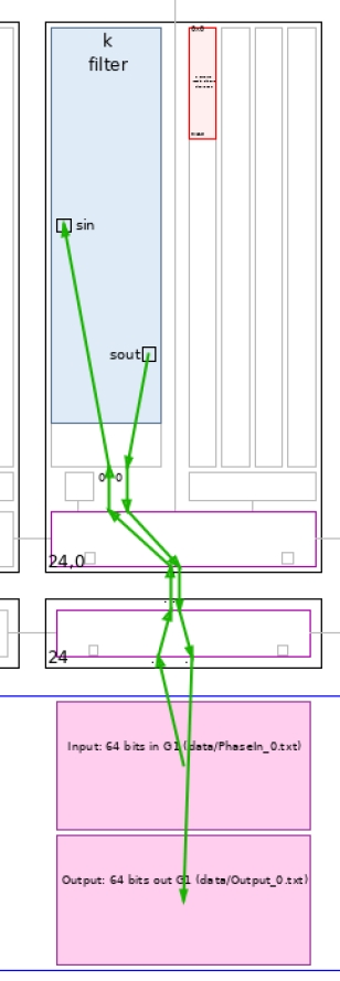
Click Array to visualize where the kernel has been placed, and how it is fed from the the PL:
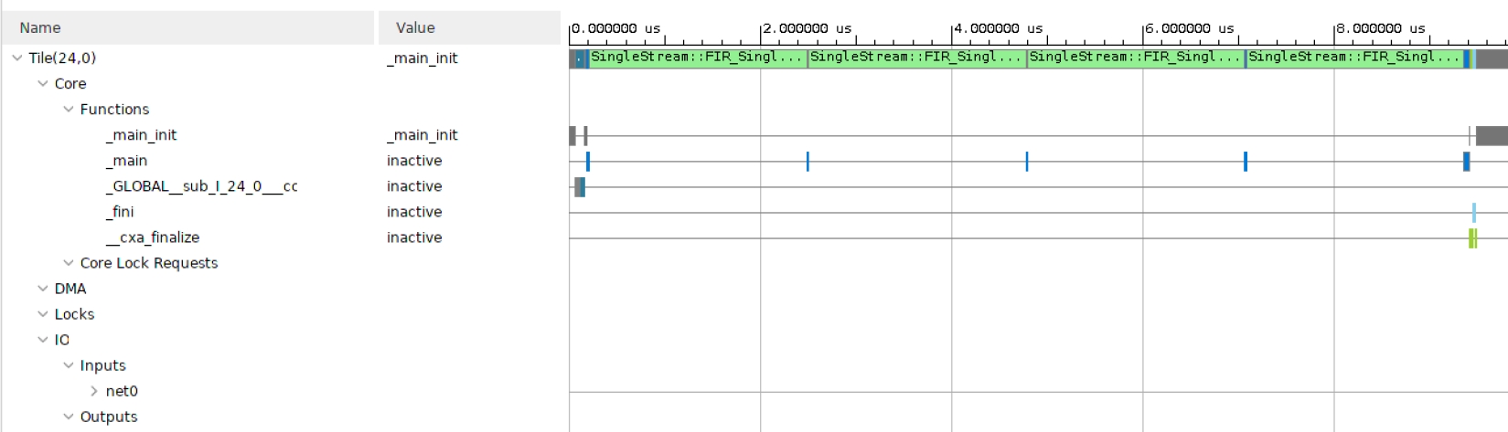
Finally click on Trace to look how the entire simulation went through. This may be useful to track where your AI Engine stalls if performance is not as expected:
As explained earlier, the directory Utils contains a number of utilities that will help in analyzing the design output. First, the output value has to be validated. The input being a set of Dirac impulses, the impulse response of the filter should be recognized throughout the waveform. Navigate to Emulation-AIE/aiesimulator_output/data and look at the Output_0.txt. You can see that you have two complex outputs per line which is prepended with a time stamp. ProcessAIEOutput Output_0.txt.
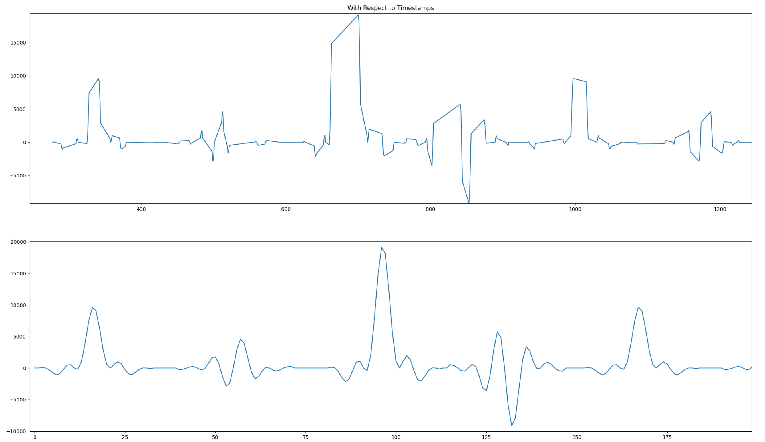
The top graph reflects the outputs where the abscissa is at the time at which this output occurred. It is much easier to look at the bottom graph where the samples are displayed one after the other. The filter impulse can be easily recognized on this sub-graph. The file out.txt contains three columns: (timestamp, real part, and imaginary part) of the output samples.
The throughput can be computed from the timeline, but a tool has been created for you in the Utils directory to compute it from the output files. In the same directory (Emulation-AIE/aiesimulator_output/data) type StreamThroughput Output_0.txt:
Output_0.txt -->   225.40 Msps

-----------------------

Total Throughput -->     225.40 Msps
Each four output samples need 16 mul4/mac4 instructions, so the maximum throughput attainable is 250 Msps which is in line with what was achieved.
Copyright© 2020–2021 Xilinx
XD020