2020.2 Vitis™ - Runtime and System Optimization
See Vitis™ Development Environment on xilinx.com
|
Overview
Looking back at the previous example, once the data grew beyond a certain size the transfer of data into and
out of our application started to become the bottleneck. Given that the transfer over PCIe will generally
take a relatively fixed amount of time, you might be tempted to create four instances of the wide_vadd
kernel and enqueue them all to chew through the large buffer in parallel.
This is actually the traditional GPU model - batch a bunch of data over PCIe to the high-bandwidth memory, and then process it in very wide patterns across an array of embedded processors.
In an FPGA we generally want to solve that problem differently. If we have a kernel capable of consuming a full 512 bits of data on each tick of the clock, our biggest problem isn’t parallelization, it’s feeding its voracious appetite. If we’re bursting data to and from DDR we can very easily hit our bandwidth cap. Putting multiple cores in parallel and operating continually on the same buffer all but ensures we’ll run into bandwidth contention. That will actually have the opposite of the desired effect - our cores will all run slower.
So what should we do? Remember that the wide_vadd kernel is actually a bad candidate for acceleration in
the first place. The computation is so simple we can’t really take advantage of the parallelism of an FPGA.
Fundamentally there’s not too much you can do when your algorithm boils down to A+B. But it does let us show
a few techniques optimizing around something that’s about as algorithmically simple as it gets.
To that end we’ve actually been a bit tricky with our hardware design for the ‘wide_vadd’ kernel. Instead of just consuming the data raw off of the bus, we’re buffering the data internally a bit using the FPGA block RAM (which is fundamentally an extremely fast SRAM) and then performing the computation. As a result we can absorb a little time between successive bursts, and we’ll use that to our advantage.
Remember that we’ve split our interfaces across multiple DDR banks, as shown in the previous example. Since the PCIe bandwidth is much lower than the total bandwidth of any given DDR memory on the Alveo™ Data Center accelerator card, and we’re transferring data to two different DDR banks, we know we’ll have interleaving between the two. And so, because we can “squeeze in between the cracks” as it were, we can start processing the data as it arrives instead of waiting for it to completely transfer, processing it, and then transferring it back. We want to end up with something like this:
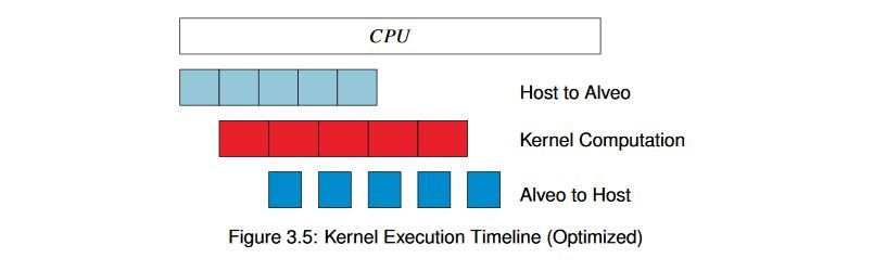
By subdividing the buffer in this way and choosing an optimal number of subdivisions, we can balance execution and transfer times for our application and get significantly higher throughput. Using the same hardware kernel, let’s take a look at what’s required to set this up in the host code.
Key Code
The algorithmic flow of the code will be mostly the same. Before queueing up transfers, we’ll loop through
the buffer and subdivide it. We want to follow a few general rules, though. First, we want to try to divide
the buffer on aligned boundaries to keep transfers efficient, and second we want to make sure we’re not
subdividing buffers when they’re so small that it makes no sense. We’ll define a constant NUM_BUFS to set
our number of buffers, and then write a new function to subdivide them:
int subdivide_buffer (std::vector<cl::Buffer> ÷d,
cl::Buffer buf_in,
cl_mem_flags flags,
int num_divisions)
{
// Get the size of the buffer
size_t size;
size = buf_in.getInfo<CL_MEM_SIZE>();
if (size / num_divisions <= 4096) {
return-1;
}
cl_buffer_region region;
int err;
region.origin = 0;
region.size = size / num_divisions;
// Round region size up to nearest 4k for efficient burst behavior
if (region.size % 4096 != 0) {
region.size += (4096 - (region.size % 4096));
}
for (inti = 0; i < num_divisions; i++) {
if (i == num_divisions - 1) {
if ((region.origin + region.size) > size) {
region.size = size - region.origin;
}
}
cl::Buffer buf = buf_in.createSubBuffer(flags,
CL_BUFFER_CREATE_TYPE_REGION,
®ion,
&err);
if (err != CL_SUCCESS) {
returnerr;
}
divided.push_back(buf);
region.origin += region.size;
}
return0;
}
What we’re doing here is looping through the buffer(s) NUM_BUFS times, calling cl::Buffer.createSubBuffer()
for each sub-buffer we want to create. The cl_buffer_region struct defines the start address and size of
the sub-buffer we want to create. It’s important to note that sub-buffers can overlap, although in our case
we’re not using them in that way.
We return a vector of cl::Buffer objects that we can then use to enqueue multiple operations, as follows:
int enqueue_subbuf_vadd(cl::CommandQueue &q,
                        cl::Kernel &krnl,
                        cl::Event &event,
                        cl::Buffer a,
                        cl::Buffer b,
                        cl::Buffer c)
{
      // Get the size of the buffer
      cl::Event k_event, m_event;
      std::vector<cl::Event> krnl_events;

      static std::vector<cl::Event> tx_events, rx_events;

      std::vector<cl::Memory> c_vec;
      size_t size;
      size = a.getInfo<CL_MEM_SIZE>();

      std::vector<cl::Memory>in_vec;
      in_vec.push_back(a);
      in_vec.push_back(b);
      q.enqueueMigrateMemObjects(in_vec, 0, &tx_events, &m_event);
      krnl_events.push_back(m_event);
      tx_events.push_back(m_event);
      if (tx_events.size() > 1) {
         tx_events[0] = tx_events[1];
         tx_events.pop_back();
      }

      krnl.setArg(0, a);
      krnl.setArg(1, b);
      krnl.setArg(2, c);
      krnl.setArg(3, (uint32_t)(size /sizeof(uint32_t)));

      q.enqueueTask(krnl, &krnl_events, &k_event);
      krnl_events.push_back(k_event);
      if (rx_events.size() == 1) {
         krnl_events.push_back(rx_events[0]);
         rx_events.pop_back ();
      }

      c_vec.push_back (c);
      q.enqueueMigrateMemObjects(c_vec,
                                 CL_MIGRATE_MEM_OBJECT_HOST,
                                 &krnl_events,
                                 &event);
      rx_events.push_back (event);

      return 0;
}
In this new function we’re doing basically the same sequence of events that we had before:
Enqueue migration of the buffer from the host memory to the Alveo memory.
Set the kernel arguments to the current buffer.
Enqueue the run of the kernel.
Enqueue a transfer back of the results.
The difference, though, is that now we’re doing them in an actual queued, sequential fashion. We aren’t
waiting for the events to fully complete now, as we were in previous examples, because that would defeat the
whole purpose of pipelining. So now we’re using event-based dependencies. By using cl::Event objects we
can build a chain of events that must complete before any subsequent chained events (non-linked events can
still be scheduled at any time).
We enqueue multiple runs of the kernel and then wait for all of them to complete, which will result in much more efficient scheduling. Note that if we had built the same structure as in Example 4 using this queuing method we’d see the same results as then, because the runtime has no way of knowing whether or not we can safely start processing before sending all of the data. As designers we have to tell the scheduler what can and cannot be done.
And, finally, none of this would happen in the correct sequence if we didn’t do one more very important
thing: we have to specify that we can use an out of order command queue by passing in the flag
CL_QUEUE_OUT_OF_ORDER_EXEC_MODE_ENABLE when we create it.
The code in this example should otherwise seem familiar. We now call those functions instead of calling the API directly from main(), but it’s otherwise unchanged.
There is something interesting, though, about mapping buffer c back into userspace - we don’t have to work
with individual sub-buffers. Because they’ve already been migrated back to host memory, and because when
creating sub-buffers the underlying pointers don’t change, we can still work with the parent even though we
have children (and the parent buffer somehow even manages to sleep through the night!).
Running the Application
With the XRT initialized, run the application by running the following command from the build directory:
./05_pipelined_vadd alveo_examples
The program will output a message similar to this:
-- Example 5: Pipelining Kernel Execution --

Loading XCLBin to program the Alveo board:

Found Platform
Platform Name: Xilinx
XCLBIN File Name: alveo_examples
INFO: Importing ./alveo_examples.xclbin
Loading: ’./alveo_examples.xclbin’

-- Running kernel test with XRT-allocated contiguous buffers and wide VADD (16 values/clock)

OCL-mapped contiguous buffer example complete!

--------------- Key execution times ---------------
OpenCL Initialization:              263.001ms
Allocate contiguous OpenCL buffers: 915.048 ms
Map buffers to userspace pointers:  0.282 ms
Populating buffer inputs:           1166.471 ms
Software VADD run:                  1195.575ms
Memory object migration enqueue:    0.441ms
Wait for kernel to complete:        692.173 ms
And comparing these results to the previous run:
| Operation | Example 4 | Example 5 | Δ4→5 |
|---|---|---|---|
| Software VADD | 820.596 ms | 1166.471 ms | 345.875 ms |
| Hardware VADD (Total) | 1184.897 ms | 692.172 ms | −492.725 ms |
| ΔAlveo→CPU | 364.186 ms | −503.402 ms | 867.588 ms |
Mission accomplished for sure this time. Look at those margins!
There’s no way this would turn around on us now, right? Let’s sneak out early - I’m sure there isn’t an “other shoe” that’s going to drop.
Extra Exercises
Some things to try to build on this experiment:
Play around with the buffer sizes again. Is there a similar inflection point in this exercise?
Capture the traces again too; can you see the difference? How does the choice of the number of sub-buffers impact runtime (if it does)?
Key Takeaways
Intelligently managing your data transfer and command queues can lead to significant speedups.
Read Example 6: Meet the Other Shoe
Copyright© 2019-2021 Xilinx