2020.2 Vitis™ - Runtime and System Optimization
See Vitis™ Development Environment on xilinx.com
|
Overview
Image processing is a great area for acceleration in an FPGA, and there are a few reasons for it. First and foremost, if you’re doing any kind of pixel-level processing as the images get larger and larger, the amount of computation goes up with it. But, more importantly, they map very nicely to our train analogy from earlier.
Let’s look at a very simple example: a bilateral resize algorithm. This algorithm takes an input image and scales it to a new, arbitrary resolution. The steps to do that might look something like this:
Read the pixels of the image from memory.
If necessary, convert them to the proper format. In our case we’ll be looking at the default format used by the OpenCV library, BGR. But in a real system where you’d be receiving data from various streams, cameras, etc. you’d have to deal with formatting, either in software or in the accelerator (where it’s basically a “free” operation, as we’ll see in the next example).
For color images, extract each channel.
Use a bilateral resizing algorithm on each independent channel.
Recombine the channels and store back in memory.
Or, if you prefer to think of it visually, the operation would look something like this:
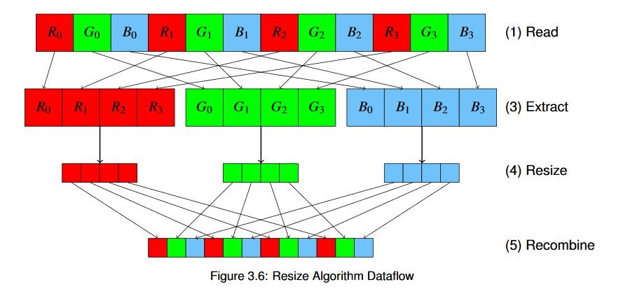
For the purposes of this diagram we haven’t shown the optional color conversion step.
The interesting thing to note here is that these operations happen one after another sequentially. Remember from our discussion earlier that going back and forth to memory is expensive. If we can perform all of these calculations in the FPGA as we stream the data in from memory, then the extra latency of each individual step or calculation will generally be extremely small. We can use that to our advantage, building custom domain-specific architectures that make optimal use of the hardware for the specific function(s) we’re trying to implement.
You can then widen the data path to process more pixels per clock - Amdahl’s Law - or you can process many images in parallel with multiple pipelines - Gustafson’s Law. Ideally, you’ll optimize on both axes: build a kernel that can process your algorithm as efficiently as possible, and then put as many kernels as you can take advantage of in the FPGA fabric.
Key Code
For this algorithm we’ll make use of the Vitis Vision libraries. These are hardware-optimized libraries implementing many commonly-used vision functions (conceptually similar to OpenCV) functions that you can directly use in your applications. We can also mix and match them with software OpenCV functions or other library calls as needed.
We can also use these libraries for image pre-and post-processing for other kernels. For example, we might want to take raw data from a camera or network stream, pre-process it, feed the results to a neural network, and then do something with the results. All of that can be done on the FPGA without needing to go back to the host memory at all, and all of these operations can be done in parallel. Imagine building a pipelined stream of functionality whose only fundamental contention is bandwidth, not register space.
In the Vitis Vision library, you configure things such as the number of pixels to process per clock, etc. via templates. I won’t go into detail here, but please refer to Vitis Vision Libraries Documentation for more information.
Running the Application
With the XRT initialized, run the application by running the following command from the build directory:
./07_opencv_resize alveo_examples <path_to_image>
Because of the way we’ve configured the hardware in this example, your image must conform to certain requirements. Because we’re processing eight pixels per clock, your input width must be a multiple of eight.
If it isn’t, then the program will output an error message informing you which condition was not satisfied. This is of course not a fundamental requirement of the library; we can process images of any resolution and other numbers of pixels per clock. But, for optimal performance if you can ensure the input image meets certain requirements you can process it significantly faster. In addition to the resized images from both the hardware and software OpenCV implementations, the program will output messages similar to this:
-- Example 7: OpenCV Image Resize --

OpenCV conversion done!  Image resized 1920 x 1080 to 640 x 360
Starting Xilinx OpenCL implementation...
Matrix has 3 channels
Found Platform
Platform Name: Xilinx
XCLBIN File Name: alveo_examples
INFO: Importing ./alveo_examples.xclbin
Loading: ’./alveo_examples.xclbin’

OpenCV resize operation:            5.145 ms
OpenCL initialization:              292.673 ms
OCL input buffer initialization :   4.629 ms
OCL output buffer initialization :  0.171 ms
FPGA Kernel resize operation :      4.951 ms
Because we’re now doing something fundamentally different, we won’t compare our results to the previous run. But we can compare the time to process our image on the CPU vs. the time it takes to process the image on the Alveo card.
For now we can notice that the Alveo card and the CPU are approximately tied. The bilinear interpolation algorithm we’re using is still O(N), but this time it’s not quite so simple a calculation. As a result we’re not as I/O bound as before; we can beat the CPU, but only just.
One interesting thing here is that we’re performing a number of computations based on the output resolution, not the input resolution. We need to transfer in the same amount of data, but instead of converting the image to 1/3 its input size, let’s instead double the resolution and see what happens. Change the code for the example as in listing 3.20 and recompile.
uint32_t out_width = image.cols*2;
uint32_t out_height = image.rows*2;
Running the example again, we see something interesting:
-- Example 7: OpenCV Image Resize --
OpenCV conversion done!  Image resized 1920 x 1080 to 3840 x 2160
Starting Xilinx OpenCL implementation...
Matrix has 3 channels
Found Platform
Platform Name: Xilinx
XCLBIN File Name: alveo_examples
INFO: Importing ./alveo_examples.xclbin
Loading: ’./alveo_examples.xclbin’

OpenCV resize operation :           11.692 ms
OpenCL initialization :             256.933 ms
OCL input buffer initialization :   3.536 ms
OCL output buffer initialization :  7.911 ms
FPGA Kernel resize operation :      6.844 ms
Let’s set aside, for a moment, the buffer initializations - usually in a well-architected system you’re not performing memory allocation in your application’s critical path. We’re now, just on the resize operation and including our data transfer, nearly 60% faster than the CPU.
While both the CPU and the Alveo card can process this image relatively quickly, imagine that you were trying to hit an overall system-level throughput goal of 60 frames per second. In that scenario you only have 16.66 ms to process each frame. If you were, for example, using the resized frame as an input into a neural network you can see that you would have almost used all of your time already.
If you’re intending to pre-allocate a chain of buffers to run your pipeline, then we’ve now regained nearly 30% of our per-frame processing time by using an accelerator.
For a 1920 x 1200 input image, we get results like this:
| Operation | Scale Down | Scale Up |
|---|---|---|
| Software Resize | 5.145 ms | 11.692 ms |
| Hardware Resize | 4.951 ms | 6.684 ms |
| ΔAlveo→CPU | −194 µs | −5.008 ms |
And the best part: remember that color conversion step I mentioned earlier? In an FPGA that’s basically a free operation - we get a few extra clock cycles (nanoseconds) of latency, but it’s fundamentally another O(N) operation, and a simple one at that with just a few multiplications and additions on the pixel values.
Extra Exercises
Some things to try to build on this experiment:
Edit the host code to play with the image sizes. How does the run time change if you scale up more? Down more? Where is the crossover point where it no longer makes sense to use an accelerator?
Add in color conversion to the FPGA accelerator (note that a hardware rebuild will be required). See if it takes longer to process.
Key Takeaways
More computationally complex O(N) operations can be good candidates for acceleration, although you won’t see amazing gains vs. a CPU
Using FPGA-optimized libraries like xf::OpenCV allows you to easily trade off processing speed vs. resources, without having to re-implement common algorithms on your own. Focus on the interesting parts of your application!
Some library optimizations you can choose can impose constraints on your design - double check the documentation for the library function(s) you choose before you implement the hardware.
We mentioned briefly earlier that doing additional processing in the FPGA fabric is very “cheap”, time-wise. In the next section let’s do an experiment to see if that’s true.
Read Example 8: Pipelining Operations with Vitis Vision
Copyright© 2019-2021 Xilinx