GQE Kernel Design
Join Kernel
The GQE join kernel is a compound of multiple post-bitstream programmable primitives, and can execute not only hash-join but also a number of primitives often found as prologue or epilogue of join operations. With its bypass design in data path, it can even perform execution without a join.
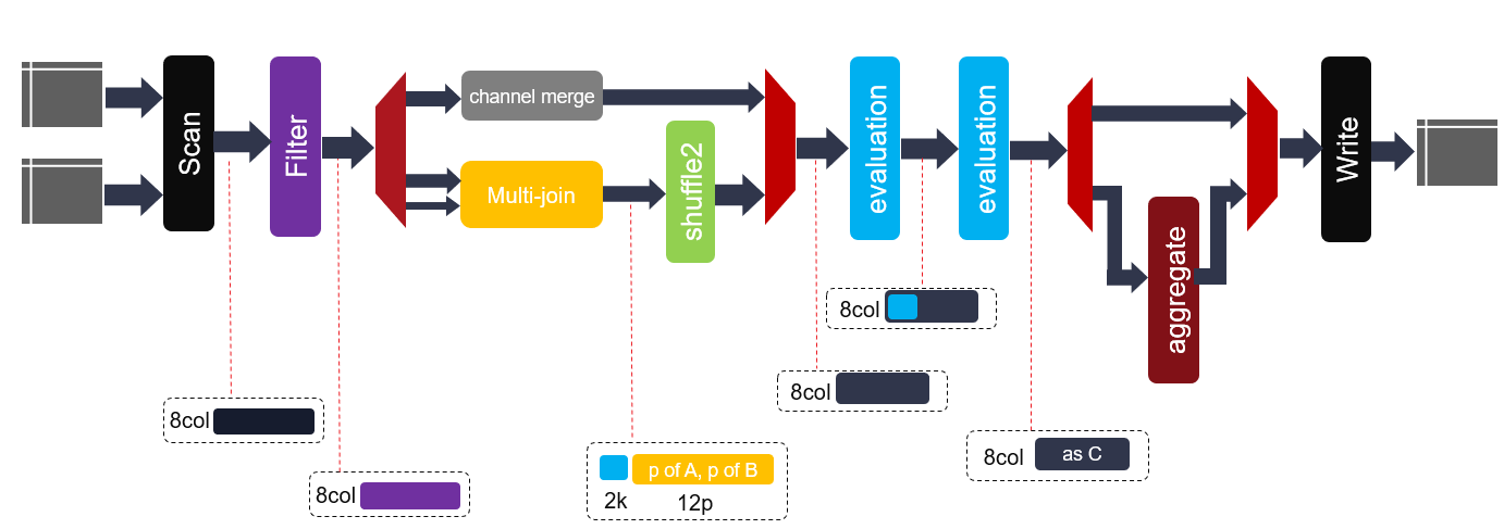
The internal of this kernel is illustrated in the figure above. Internal multi-join supports three reconfigurable modes, namely inner join, anti-join and semi-join. This kernel works with three input buffers, two for data and one for configuration, and it emits result to one output buffer, with same data structure as its data input buffers.
The uniformed buffer content structure design allows this kernel to be seamlessly scheduled, using one’s output as successor’s input. Basically, a buffer contains an input table or an intermediate result table, and each table has a list of data columns, placed one after another and aligned to 512b boundaries.
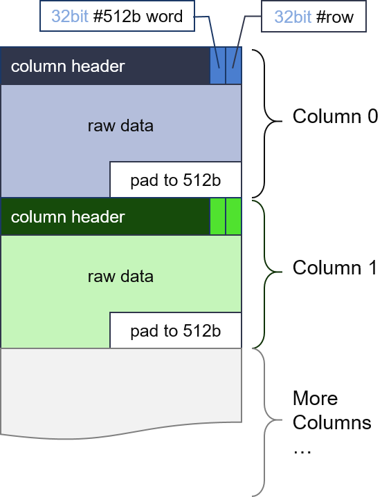
Each column’s data structure is essentially a 512-bit header, followed by raw data.
Note
In the current release, all columns are expected to have the same number of elements of same type, so only the first columns header is used by kernel. This will likely change in future release.
The buffer and column’s data structure is shown in the figure below.
The configuration buffer basically programs the kernel at runtime. It toggles execution step primitives on or off, and defines the filter and/or evaluation expressions. The details are documented in the following table:
| 192-511 | 191-184 | 120-183 | 56-119 | 6 | 3-5 | 2 | 1 | 0 |
|---|---|---|---|---|---|---|---|---|
| Shuffle | Tab C col sel | Tab B col-id | Tab A col-id | append | join sel | dual key | aggr on | join on |
| (padding at MSB) eval-0 config | ||||||||
| (padding at MSB) eval-1 config | ||||||||
| filter Tab A config | ||||||||
| filter Tab A config (cont’) | ||||||||
| (padding at MSB) filter Tab A config (cont’) | ||||||||
| filter Tab B config | ||||||||
| filter Tab B config (cont’) | ||||||||
| (padding at MSB) filter Tab B config (cont’) | ||||||||
Both input table A and B can support up to 8 columns.
The selection and order of columns in pipeline is appointed via the column index.
Within each buffer, the columns are indexed starting from 0.
-1 is used as a special value to instruct the table scanner to feed zero for that column.
For example, suppose Table A’s column indices are [3,2,1,-1,-1].
Then Column 3 will be the first in data path, and Column 2 the second and Column 1 the third.
Column 0 and other columns if exists are ignored.
The last two slots in data path will be filled with zeros.
The filter config is aligned to lower bits, and each filter’s config fully covers the first two 512-bit slots, and partially use the third one.
Here the join_on option toggles whether hash-join is enabled or by-passed in the pipeline.
The dual_key option instructs the kernel to use
both first and second column as join key in hash-join, and when it is asserted, the third column
becomes the first part of the payload input.
The join sel option indicates the work mode of multi-join, 0 for normal hash join, 1 for semi-join and
2 for anti-join.
The append option toggles whether the append mode is enabled during writing out consecutive joined table.
This option would be usually used when it joins two sub-tables after hash partition.
The eval config is for the dynamicEval primitive, and aligns to the lower bits of the 512-bit allocated for it.
The aggregation always performs the calculation of min, max, sum and count for each of its input column.
When aggr_on is set, aggregation values will write instead of the original rows.
Caution
To support large sum and count, the output data width of these two fields are doubled.
So that the aggregation value for each column is min, max, sum LSB, sum MSB, count LSB, count MSB.
The write option is basically a bit mask for 8 slots in data path. Only when the corresponding one-hot bit is asserted, the column is written to the output buffer.
Caution
Due to limitation in current write_out, the output buffer must always
provide 8 column slots, even not all used.
The hardware resource utilization of join kernel is shown in the table below (work as 182MHz).
| Primitive | Quantity | LUT | LUT as memory | LUT as logic | Register | BRAM36 | URAM | DSP |
| Scan | 1 | 12814 | 4758 | 8056 | 18968 | 0 | 0 | 2 |
| Filter | 4 | 2155 | 13 | 2142 | 1776 | 0.5 | 0 | 0 |
| Hash join | 1 | 118625 | 30396 | 88229 | 171852 | 254.5 | 192 | 80 |
| Eval | 2 | 2362 | 315 | 2047 | 2325 | 0 | 0 | 21 |
| Direct aggr | 1 | 1958 | 0 | 1958 | 3307 | 0 | 0 | 0 |
| Write | 1 | 20604 | 5693 | 14911 | 30275 | 0 | 0 | 0 |
| AXI DDR | 1 | 6803 | 1370 | 5433 | 15045 | 60 | 0 | 0 |
| AXI HBM | 1 | 25734 | 3321 | 22413 | 31290 | 32 | 0 | 0 |
| Total | 236692 | 63384 | 173608 | 330108 | 348.5 | 192 | 124 |
Aggregate Kernel
The GQE Aggregate kernel is another key kernel of General Query Engine (GQE), and supports both grouping and non-grouping aggregate operations.
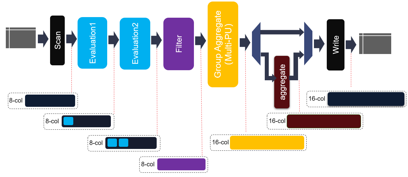
The internal structure of this kernel is shown in the figure above. It consists of one scan and write, two evaluations, one filter, hash group aggregate as well as one aggregate primitive. Raw input table is scanned in or write out by column. Before entering into hash group aggregate module, each element in each row will be evaluated and filtered. Thus, some new elements can be generated and some rows will be discarded behind. Moreover, two cascaded evaluation modules are added to support more complex expression.
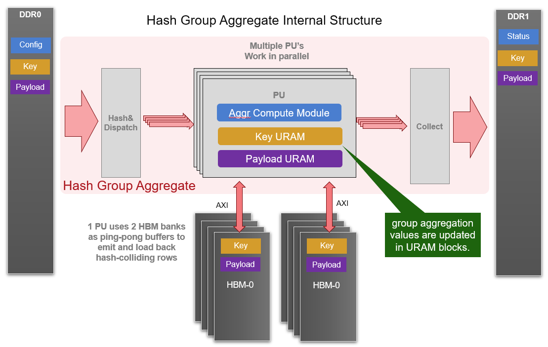
Hash group aggregate is the key module in this kernel, which is a multi-PU implementation and given in the following diagram. Each PU requires 2 HBM banks and some URAM memory blocks to buffer distinct keys as well as payloads after aggregate operations. And one internal loop is implemented to consume all input rows with each iteration. Furthermore, all PUs are working in parallel to achieve higher performance.
Also, the data structure of input and output tables is same as join kernel. The whole configuration is composed of 128 32-bit slot. And the details of configuration buffers are listed in the table:
| Module | Module Config Width | Position |
| Scan | 64 bit | config[0]~config[1] |
| Eval0 | 289 bit | config[2]~config[11] |
| Eval1 | 289 bit | config[12]~config[21] |
| Filter | 45*32 bit | config[22]~config[66] |
| Shuffle0 | 64 bit | config[67]~config[68] |
| Shuffle1 | 64 bit | config[69]~config[70] |
| Shuffle2 | 64 bit | config[71]~config[72] |
| Shuffle3 | 64 bit | config[73]~config[74] |
| Group Aggr | 4*32 bit | config[75]~config[78] |
| Column Merge | 64 bit | config[79]~config[80] |
| Aggregate | 1 bit | config[81] |
| Write | 16 bit | config[82] |
| Reserved | config[83]~config[127] |
The hardware resource utilization of hash group aggregate is shown in the table below (work as 193MHz).
| Primitive | Quantity | LUT | LUT as memory | LUT as logic | Register | BRAM36 | URAM | DSP |
| Scan | 1 | 12209 | 4758 | 7451 | 18974 | 0 | 0 | 2 |
| Eval | 8 | 2153 | 426 | 1727 | 2042 | 4 | 0 | 21 |
| Filter | 4 | 2168 | 13 | 2155 | 1764 | 0.5 | 0 | 0 |
| Group Aggr | 1 | 162202 | 27819 | 134383 | 210926 | 62 | 256 | 0 |
| Direct Aggr | 1 | 4349 | 0 | 4349 | 6611 | 0 | 0 | 0 |
| Write | 1 | 30938 | 9490 | 21448 | 43579 | 0 | 0 | 0 |
| AXI DDR | 1 | 4586 | 1313 | 3273 | 78855 | 18 | 0 | 0 |
| AXI HBM | 1 | 20528 | 4456 | 16072 | 45416 | 124 | 0 | 0 |
| Total | 298470 | 60402 | 238068 | 399737 | 255 | 256 | 2 |
Partition Kernel
The GQE partition kernel can partition one table’s rows into corresponding clusters according to hash of selected key columns. This kernel is designed to scale the problem size that can be handled by the GQE Join or Aggregate kernel. To reduce the size of intermediate data, it is equipped with dynamic filter like other kernels.
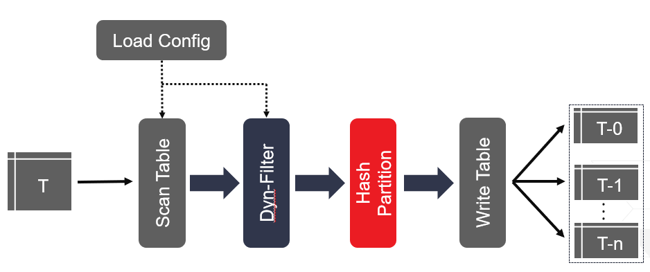
The internal of this kernel is illustrated in the figure above. It consists of two input buffers and one output buffer. Firstly, the kernel scans the input tables into multiple columns and then it filters them (if the related condition is given in configuration buffer). After that, each row will be dispatched into various buckets based on the hash value of primary key. Finally, every full hash bucket will trigger on one burst write into output buffer.
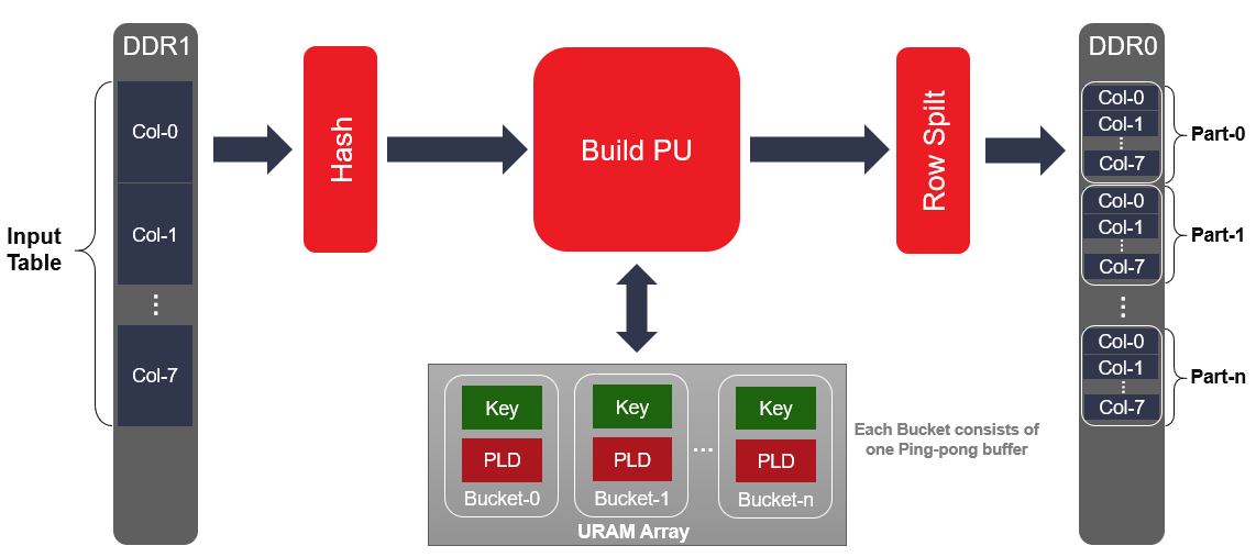
The details for hash partition is shown in the following figure. One URAM array is used to buffer one burst length rows for each hash part. And the following module behind build PU will spilt each row into multiple columns for compatible output format with other kernels.
To simplify the design, GQE partition kernel can reuse the scan and filter configuration with GQE join kernel. Also, as mentioned above, the data structure of input and output tables is the same as join kernel.
The hardware resource utilization of single hash partition is shown in the table below (work as 200MHz).
| Primitive | Quantity | LUT | LUT as memory | LUT as logic | Register | BRAM36 | URAM | DSP |
| Scan | 1 | 12032 | 4752 | 7280 | 19383 | 0 | 0 | 2 |
| Filter | 4 | 3551 | 809 | 2742 | 3809 | 0.5 | 0 | 0 |
| Hash partition | 1 | 26363 | 1521 | 27496 | 45762 | 20 | 256 | 5 |
| Write | 1 | 26083 | 5082 | 21286 | 33202 | 1 | 0 | 3 |
| AXI DDR | 1 | 5046 | 1010 | 4036 | 11303 | 59.5 | 0 | 0 |
| Total | 76091 | 14102 | 61989 | 116884 | 81 | 256 | 10 |
Attention
To use the GQE Partition kernel, host must pass the number of partitions through a kernel argument, create corresponding number of sub-buffers on Partition kernel’s output, and invoke GQE Join or Aggregate kernel multiple times accordingly.