GQE L3 Design
Overview
The GQE L3 APIs, which schedule the kernel execution, data transfers, and CPU data movement in pipeline, hides the detailed OpenCL calls, are provided for software programmers. Three categories of soft APIs are implemented, including join, bloom-filter, and group-by aggregate. Joiner and Bloomfilter are polished to supports 64-bit data input/output in this release. Aggegator kept 32-bit data input/output which is the same as the 2020.2 release.
Joiner Design
Join has two phases: build and probe. When the build table is fixed, the probe efficiency is linear to probe table size. However, when the build table gets larger, the performance of the probe decreases. In real scenarios, the size of both build and probe table is unknown. Therefore, to support different sized two tables’ join with efficient performance, two solutions are provided in L3:
- solution 0/1: Direct Join (1x Build + Nx Probe), which is used when the build table is not too large.
- solution 2: Hash Partition + Hash Join, partitioning left table and right table to M partitions. Thereafter, Perform Build + Nx Probe for each partition pair.
In solution 1, the size of the build table is relatively small, so the probe phase is efficient. To minimize the overhead of data transfer and CPU data movement, the probe table is splitted into multi-section horizontally.
When the build table is large, partitioning the input tables into multi-partitions may keep the high-performance execution of build+probe. Solution 2 includes three sequential phases: Partitioning build table O, partitioning probe table L, and do multiple times of solution 1. For each phase, pipelined task scheduling is employed.
Note
Comparing these two type of solutions, although partitioning table O and L introduces extra overhead of partitioning, the build+probe time is decreased due to the dramatically reduced unique key radio.
Caution
With TPC-H Q5s query as the example, the solution 1 and 2 switching data size for build table is ~ SF8 (confirm?). Which is to say, when the scale factor is smaller than SF8, solution 1 is faster. For datasets larger than SF8, solution 2 would be faster.
Workshop Design
Workshop consist of the following 3 parts:
- A vector of Worker: each Worker instance will manage 1 Alveo card and managed device buffers their host mapping pinned buffers. They will handle 1) migration of input data from pinned memory to device memory, 2) kernel arguments setup and kernel call, 3) migration of meta data from device memory to pinned memory, 4) migration of result data from device memory to pinned memory based on meta data.
- 1 MemCoppier, from host to pinned : has 8 threads to performance memcpy task from input memory to host mapping pinned buffer.
- 1 MemCoppier, from pinned to host : has 8 threads to performance memcpy task from input memory to host mapping pinned buffer.
Workshop’s constructor will find all cards with the same desired shell, and load them with the xclbin files provided. After the constructor is done, it will create same number of worker with cards for managements. The openCL related context, program, kernel, command queue will only be released if the release function is called.
Workshop support to performance Join on multiple cards, with asynchronous input and output. Please take reference of L3/tests/gqe/join case as example of how to notify readiness of each input section and how to wait for readiness of output sections.
Workshop support two solultions for Join. Solution 1 is like Joiner’s solution 1, solution 2 is like Joiner’s solution 2. It does not provide standalone solution 0 because it is could be covered by solution 1. Workshop will handle task distribution between workers so this will be transparent to caller.
Bloom-Filter Design
Class specifications
Generally, we provide 3 L3 classes for GQE Bloom-Filter to alleviate the software developers’ suffering for calling OpenCL APIs, arranging the column shuffles, splitting the table into sections with excutable size to accelerate database queries with the hardware kernels:
gqe::FilterConfig: for generating software shuffles for input and output columns plus the kernel configuration bits.gqe::BloomFilter: for calculating the bloom-filter size based on the number of unique keys, allocating buffers for internal hash-table, and performing software build and merge processes as we currently do not support build process for bloom-filtering.gqe::Filter: for performing the multi-threaded pipelined bloom-filtering.
Example Usage
Since programming the FPGA is very time-consuming, we provide the hardware initialization and hardware run processes independently.
For initializing the hardware:
// Initializes FPGA
gqe::FpgaInit init_ocl(xclbin_path);
// Allocates pinned host buffers
init_ocl.createHostBufs();
// Allocates device buffers
init_ocl.createDevBufs();
For loading the table columns and building the bloom-filter’s hash-table:
// Please first load data to corresponding table L column buffers
// We assume input table columns is stored in tab_l_col0 & tab_l_col1,
// and the corresponding number of rows is stored in table_l_nrow

const int BUILD_FACTOR = 10;
using namespace xf::database;

// Builds 0 - 1/BUILD_FACTOR of table L into bf1
for (int i = 0; i < table_l_nrow / BUILD_FACTOR; i++) {
    tab_o1_col0[i] = tab_l_col0[i];
    tab_o1_col1[i] = tab_l_col1[i];
}

// Builds 1/BUILD_FACTOR - 2/BUILD_FACTOR of table L into bf2
for (int i = table_l_nrow / BUILD_FACTOR; i < (table_l_nrow / BUILD_FACTOR) * 2; i++) {
    tab_o2_col0[i - table_l_nrow / BUILD_FACTOR] = tab_l_col0[i];
    tab_o2_col1[i - table_l_nrow / BUILD_FACTOR] = tab_l_col1[i];
}

// Total number of unique keys at maximum
uint64_t total_num_unique_keys = table_l_nrow / BUILD_FACTOR * 2;

// Creates L table
gqe::Table tab_l("Table L");
tab.addCol("l_orderkey", gqe::TypeEnum::TypeInt64, tab_l_col0, table_l_nrow);
tab.addCol("l_extendedprice", gqe::TypeEnum::TypeInt64, tab_l_col1, table_l_nrow);

// Creates O1 table for building bloom-filter-1
gqe::Table tab_o1("Table O1");
tab_o1.addCol("l_orderkey", gqe::TypeEnum::TypeInt64, tab_o1_col0, table_l_nrow / BUILD_FACTOR);
tab_o1.addCol("l_extendedprice", gqe::TypeEnum::TypeInt64, tab_o1_col1, table_l_nrow/ BUILD_FACTOR);

// Builds bloom-filter-1
gqe::BloomFilter bf1(total_num_unique_keys);
bf1.build(tbl_o1, "l_orderkey");

// Creates C table for stroing filtered results, at worst, we'll get every input key passes through the bloom-filter,
// so the size of the table c should be the same with table L
gqe::Table tab_c("Table C");
tab_c.addCol("c1", gqe::TypeEnum::TypeInt64, tab_c_col0, table_l_nrow);
tab_c.addCol("c2", gqe::TypeEnum::TypeInt64, tab_c_col0, table_l_nrow);
Some use cases may need to merge several bloom-filters before running the filtering process:
// Creates O2 table for building bloom-filter-2
gqe::Table tab_o2("Table O2");
tab_o2.addCol("l_orderkey", gqe::TypeEnum::TypeInt64, tab_o2_col0, table_l_nrow / BUILD_FACTOR);
tab_o2.addCol("l_extendedprice", gqe::TypeEnum::TypeInt64, tab_o2_col1, table_l_nrow/ BUILD_FACTOR);

// Builds bloom-filter-2
gqe::BloomFilter  bf2(total_num_unique_keys);
bf2.build(tab_o2, "l_orderkey");

// Merges bloom-filter-2 into bloom-filter-1
bf1.merge(bf2);
At last, call the run API of gqe::Filter to perform the pipelined bloom-filtering:
// Creates bloom-filter engine
gqe::Filter bigfilter(init_ocl);
// Creates StrategySet object to pass on the number of sections of the table
gqe::StrategySet params;
// if set to 0, the section info should be provided in table L
// if set to n (n > 0), the table L should be divided into n sections evenly
params.sec_l = 1;
gqe::ErrCode err_code;
// Performs the bloom-filtering
err_code = bigfilter.run(tab_l // input talbe
                         "l_orderkey", // selects key from input table
                         bf1, // bloom-filter which provides hash-table
                         "",  // dynamic filter condition, empty for all passes through
                         tab_c, // output table
                         "c1=l_extendedprice, c2=l_orderkey", // output mapping
                         params); // Parameter strcut to provide section info
Group-By Aggregate Design
Caution
No updates from Aggregate kernel and L3 Aggregate API. The 2020.2 released gqePart-32bit + gqeAggr-32bit kernel are employed here.
In L3 Aggregation, all solutions are listed below:
- solution 0: Hash Aggregate, only for testing small datasets.
- solution 1: Horizontally Cut + Pipelined Hash Aggregation
- solution 2: Hash Partition + Pipelined Hash aggregation
In solution 1, the first input table is horizontally cut into many slices, then do aggregation for each slice, finally merge results. In solution 2, the first input table is hash partitioned into many hash partitions, then do aggregation for each partition (no merge in last). Comparing the two solutions, solution 1 introduces extra overhead for CPU merging, while solution 2 added one more kernel(hash partition) execution time. In summary, when input table has a high unique-ratio, solution 2 will be more beneficial than solution 1. After profiling performance using inputs with different unique key ratios, we get the turning point.
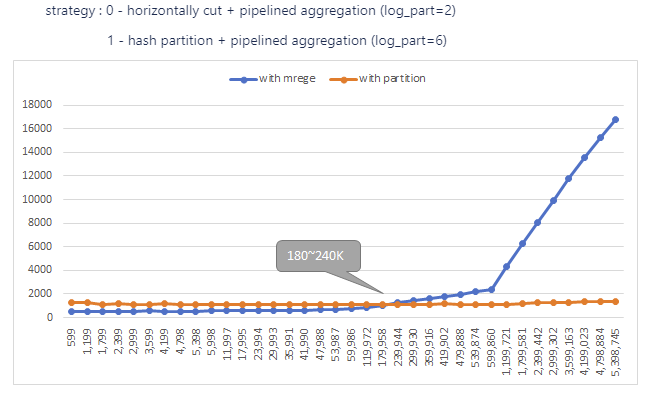
In this figure, it shows when the unique key number is more than 180K~240K, we can switch from solution 2 to solution 3.
Others: 1) Hash Partition only support max 2 keys, when grouping by more keys, use solution 2 2) In solution 1, make one slice scale close to TPC-H SF1. 3) In solution 2, make one partition scale close to TPC-H SF1.