Vitis Database Library Tutorial
Relational Database and Hardware Acceleration
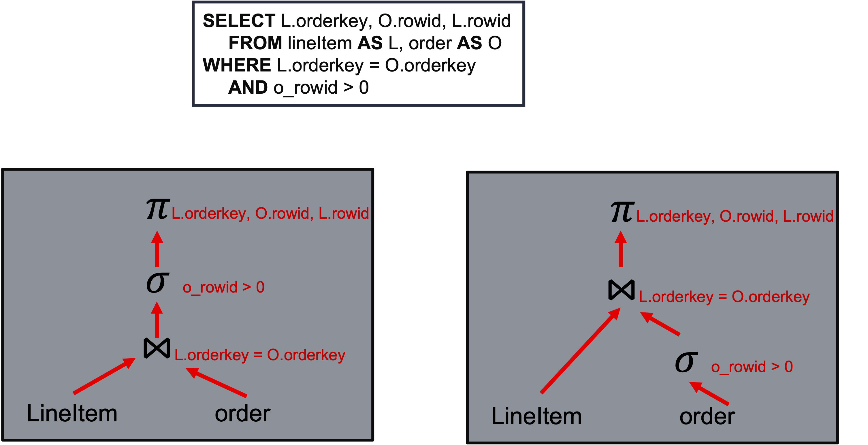
Relational databases are based on relational model of data which is powerful and used for a wide variety of information. Users only need to specify the result they want with a query language like SQL. DBMS converts a query into an execution plan which is a tree of operators, based on certain set of rules and cost functions. Execution of the plan is that data flows from the leaves towards the root and the root node produce the final result. Query execution performances depend on both execution plan and performance of operator nodes.
Xilinx Alveo card can help improve operator performance in following ways:
- Instruction parallelism by creating a customized and long pipeline.
- Data parallelism by processing multiple rows at the same time.
- Customizable memory hierarchy of BRAM/URAM/HBM, providing high bandwidth of memory access to help operators like bloom filter and hash join.
How Vitis Database Library Works
Vitis database library targets to help SQL engine developers to accelerate query execution. It provides three layers of APIs, namely L1 / L2 / L3. Each tackles different parts of the whole processing.
- L3 provide pure software APIs for:
- Define data structures to describe input table / output table / operation types and parameters.
- Provide combination of operations for acceleration. These combinations are commonly used and easy to fit into the whole execution plan.
- Manage multiple FPGA cards automatically, including initialization of OpenCL context, command queue, kernels and buffers.
- Break down incoming job, distributing sub jobs among all FPGA cards, pipeline data transfers and kernel executions.
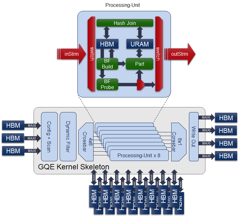
- L2 APIs are kernels running on FPGA cards. Each time called, they will finish certain processing according to input configs. L2 APIs are combinations of multiple processing units, each unit consists of multiple processing stages. In this way, kernels could both process multiple data at the same time and apply multiple operations to the same data. L2 API design is subject to resource constraints and may differs according to FPGA cards.
- L1 APIs are basic operators in processing, like filter, aggregator / bloom filter / hash join. They’re all highly optimize HLS design, providing optimal performance. They’re all template design, make them easier to scale and fit into different resource constraint.
L3 API – General Query Engine
Target Audience and Major Features
Target audience of L3 API (General Query Engine, GQE) are users who just want to link a shared library and call the API to accelerate part of execution plan on FPGA cards.
The major feature of L3 API are:
- Generalized query execution. L3 API pre-defined operator combinations like “scan + filter + aggregation + write”, “scan + filter + bloom filter + write”, “scan + filter + hash-join + write”, “scan + filter + aggregation + write”. Filter condition support comparision between 4 input columns and 2 constants. Aggregation support max / min / sum / count / mean / variance / norm_L1 / norm_L2. In this way, L3 API could support a generalized query operators.
- Automatic card management. As soon as program created an instance of GQE, it will scan the machine and find all qualified Xilinx FPGA cards by their shell name. It will load the cards with the xclbins, create context / command queue / kernel / host buffer / device buffer / job queue for each card. It will keep alive until user call release() functions. This will finish all the initialization automatically and save the overhead to repeat such setup each time user call GQE API.
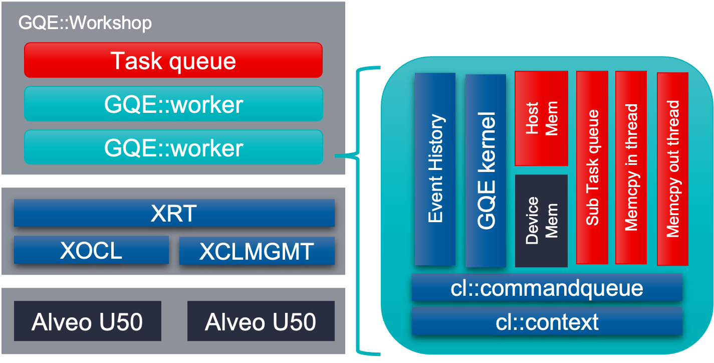
- Light weight memory management. The input and output of GQE are data structure call “TableSection”. It only contains pointers to memories which user allocated. In such way, GQE won’t do memory allocation related to input / output. This will make it easier for customer to integrate since it won’t impact original DBMS’s memory pool managment.
- Asynchronous API call. Input for processing will be cut into multiple section of rows. GQE API requries customer to provide an std::future type argument for each row, to indicate readiness of input. GQE also requires an std::promise type argument for each output section, to notify the caller thread that result is ready. GQE API will push all input arguments into an internal job queue and return immediately. Actual processing won’t begin until the corresponding std::future arguments for input is ready. This will seperate input preparing from actual GQE processing. GQE could start processing the ready sections ahead even if not all input sections are ready. It will help pipeline the “preparing” and “processing” and improve system performance.
- Column-oriented. Columnar DBMS will benefit from only accessing subset of columns and more options for data compression.
Example Usage
// Take the short query above to demonstrate how to use L3 APIs.

// create GQE instance to handle card management
// with shell name, path to xclbin file to be loaded, operator combination
gqe::workshop wksp("xilinx_u280_xdma_201920_3", "./gqe_join.xclbin", gqe::WorkerFunctions::JOIN);

// Define input table schema, including attributes and size of each attribute's element.
// Also setup if enable rowid and validation bits or not.
// rowid is an auto generated attribute inside kernel.
// validation bits represent if valid for each input rows.
// Table O has 1 column, of type int64_t, attribute name is "o_rowid", rowID and validation bits enabled, attribute name is "o_rowid", "o_valid"
// Table L has 1 column, of type int64_t, attribute name is "l_rowid", rowID and validation bits enabled, attribute name is "l_rowid", "l_valid"
// Table C has 3 column, of type int64_t, attribute name is "c1", "c2", "c3", has no rowid and validation bits"
gqe::TableSection tab_o("Table O", {"o_orderkey"}, {sizeof(int64_t)}, 1, valid_o, "o_rowid", "o_valid");
gqe::TableSection tab_l("Table L", {"l_orderkey"}, {sizeof(int64_t)}, 1, valid_l, "l_rowid", "l_valid");
gqe::TableSection tab_c("Table C", {"c1", "c2", "c3"}, {sizeof(int64_t), sizeof(int64_t), sizeof(int64_t)}, 0, 0, "", "");

// After the schema of input table has been defined, add rows by section.
// Each section added to TableSection should contains exactly same number of columns in the exact same order of attribute.
// This only add pointers, which should been valid no later than this section's corresponding future is ready.
// tab_o_col0, tab_l_col0, tab_c_col0, tab_c_col1, tab_c_col2, tab_c_col3 are pointer to input and output memory
// tab_o_valid, tab_l_valid is the validation bits for table O and table L, represent filter result from previous processing, as input.
// tab_part_o_col0, tab_part_l_col0 are pointer to intermediate partition result.
tab_o.addSec(vector<char*>({(char*)tab_o_col0}), tab_o_valid, table_o_nrow);
tab_l.addSec(vector<char*>({(char*)tab_l_col0}), tab_l_valid, table_l_nrow);
tab_c.addSec(vector<char*>({(char*)tab_c_col0, (char*)tab_c_col1, (char*)tab_c_col2, (char*)tab_c_col3}, nullptr, table_c_nrow);
tab_part_o.addSec(vector<char*>({(char*)tab_part_o_col0}), nullptr, table_o_nrow * 2);
tab_part_l.addSec(vector<char*>({(char*)tab_part_l_col0}), nullptr, table_l_nrow * 2);


// intermeidiate result will be stored in "tab_part_o" and "tab_part_l".
// schema definition and adding section are similar
gqe::TableSection tab_part_o("Part O", {"o1", "o2", "o3"}, {sizeof(int64_t), sizeof(int64_t), sizeof(int64_t)}, 0, 0, "", "");
gqe::TableSection tab_part_l("Part L", {"l1", "l2", "l3"}, {sizeof(int64_t), sizeof(int64_t), sizeof(int64_t)}, 0, 0, "", "");
tab_part_o.addSec({((char*)tmp_o1), ((char*)tmp_o2), ((char*)tmp_o3)}, nullptr, d_part_o_nrow);
tab_part_l.addSec({((char*)tmp_l1), ((char*)tmp_l2), ((char*)tmp_l3)}, nullptr, d_part_l_nrow);

// Call GQE API to perform "filter + hash partition + hash join"
// This will merge the original execution plan tree into 1 operations.
// Table O is filtered with "o_rowid>0"
// No filter and only partition on table L.
// To support bigger input tableSection, GQE will also perform hash partition on Table O and Table L.
// Join table O and table L with "o_orderkey = l_orderkey", output 3 columns of l_orderkey, o_rowid and l_rowid.
// Join will return imediately
wksp.Join(&tab_o, "o_rowid>0", &tab_o_ready, &tab_part_o, &tab_l, "", &tab_l_ready, &tab_part_l,
      "o_orderkey = l_orderkey", "c1=l_orderkey,c2=o_rowid,c3=l_rowid", &tab_c, &tab_c_ready_promise,
      gqe::INNER_JOIN, smanual);

// get future from promise
std::future<size_t> tab_c_ready;
tab_c_ready = tab_c_ready_promise.get_future();
// wait for future
tab_c_ready.get();

// release GQE
wksp.release();
L2 API – GQE kernels
Target Audience and Major Features
The target audience of L2 API are users who have a certain understanding of HLS and programming on FPGA and want to make modifications on kernels, including:
- Operator combinations in the kernel, like the number of operators or operator pipeline. Most L1 APIs and glue logics inside L2 kernels are connected with streams. Users could add more operators into kernels to increase its performance as long as it is not bounded by other factors like logic resource and memory bandwidth.
- Add more pre-processing and post-processing to kernel, like compression / decompression. Certain DBMS might store its data in compressed format to save the memory space and bandwidth to transfer. Adding decompression module to build longer processing pipeline will save the time to decompress the data and increase system performance.
- Kernel combination to be built on single cards. People might be interested in adjusting the kernel combination to accelerate the execution plan with different weights.
- Building configs to improve frequency or migrate to other Xilinx FPGA device.
- Test correctness in sw-emu, hw-emu and on-board.
Command to Run L2 cases
cd L2/tests/vitis_case_folder

# build and run one of the following using U280 platform
make run TARGET=sw_emu DEVICE=/path/to/xilinx_u280_xdma_201920_3.xpfm

# delete generated files
make cleanall
Here, TARGET decides the FPGA binary type
sw_emuis for software emulationhw_emuis for hardware emulationhwis for deployment on physical card. (Compilation to hardware binary often takes hours.)
Besides run, the Vitis case makefile also allows host and xclbin as build target.
L1 API
Target Audience and Major Features
Target audience of L1 API are users who is familiar with HLS programming and want to test / profile / modify operators or add new operator. With the HLS test project provided in L1 layer, user could get:
- Function correctness tests, both in c-simulation and co-simulation
- Performance profiling from HLS synthesis report and co-simulaiton
- Resource and timing from Vivado synthesis.
Command to Run L1 cases
cd L1/tests/hls_case_folder

make run CSIM=1 CSYNTH=0 COSIM=0 VIVADO_SYN=0 VIVADO_IMPL=0 \
    DEVICE=/path/to/xilinx_u280_xdma_201920_3.xpfm
Test control variables are:
CSIMfor high level simulation.CSYNTHfor high level synthesis to RTL.COSIMfor co-simulation between software test bench and generated RTL.VIVADO_SYNfor synthesis by Vivado.VIVADO_IMPLfor implementation by Vivado.
For all these variables, setting to 1 indicates execution while 0 for skipping.
The default value of all these control variables are 0, so they can be omitted from command line
if the corresponding step is not wanted.