RTM Introduction
Reverse Time Migration (RTM) is an important seismic imaging technique used for producing an accurate representation of the subsurface. It has been adopted by the oil and gas industry for many years. However, the high computation demand, the high memory storage requirement and the less cache-friendly memory access pattern present a significant challenge. The region under detection, in general, is a 3 dimentional field with each direction few kilometers. In some special situation, the problme is simplified to a 2 dimentional field by assuming the uniformity along one direction.
Mathematics in RTM
1. Wave equation and the finite difference method
Equation (1) is the basic mathematical equation for elastic wave propagation.
where \(\nabla^2\) is the Laplace operator, \(p(\mathbf{x}, t)\) is the wave field and \(v(\mathbf{x})\) is the wave velocity. In 2D-RTM, \(\mathbf{x} = \{x, z\}\), which is the length and depth of the imaging area respectively. In 3D-RTM, \(\mathbf{x} = \{x, y, z\}\), which is the length, width and depth of the imaging area respectively.
Due to the non-uniform structures in the subsurface, there is no theoretical solution for Equation 1. Hence, RTM is based on a numerical solution called a finite difference method. All spacial dimensions and time domains are discretized properly. The partial derivative with respect to time and the Laplace operator also have corresponding transformation according to the discretization scheme.
For instance, the Pluto synthetic seismic velocity model which was used to evaluation our 2D-RTM implementation has been discretized into a regular grid both spatially and temporally. The number of partiitions are listed in Table 1.
| Parameter | Length (\(N_{x}\)) | Depth (\(N_{z}\)) | Time (\(N_{t}\)) |
| No. grids | 6960 | 1201 | 12860 |
where \(N_x\), \(N_z\), \(N_t\) denote the number of grids along \(x\), \(z\), \(t\) respectively.
Similar to the approaches presented in many research publications, we also adopted Order-2 temporal scheme and Order-8 spatial scheme. Following these discretization schemes, the 2D wave equation can be re-interpreted by Equation (2) and (3) shown below. Equation (2*) and (3) are for 3D RTM.
Where all \(c_n\) are the coeffients shown in Table 2 below.
| \(c_{4}\), \(c_{-4}\) | \(c_{3}\), \(c_{-3}\) | \(c_{2}\), \(c_{-2}\) | \(c_{1}\), \(c_{-1}\) | \(c_{0}\) |
| \(-\frac{1}{560}\) | \(\frac{8}{315}\) | \(-\frac{1}{5}\) | \(\frac{8}{5}\) | \(-\frac{1}{560}\) |
2. Imaging
The seismic imaging is via cross-correlation between a source wavefield and a receiver wavefield. Mathematically, it can be expressed as Equation 4.
where \(N_s\) is the total number of shots, \(p_s^i(\mathbf{x}, t_n)\) is a source wavefield and \(p_r^i(\mathbf{x}, t_n)\) is a receiver wavefield.
3. Boundary saving scheme
To correctly reconstruct the source wavefield in the backward process, it is necessary to extend the boundary and save the boundaries value in a forward process. For 2D-RTM, there are 4 boundaries to deal with. Dussaud [1] et al. proposed saving half-order length of all the 4 boundaries with absorbing boundary condition. In this case, the reconstruction source wavefield is definitely perfect. However, a huge amount of storage is required. In our project, we adopt the scheme proposed by Liu [2] which saved only half-order length of the upper boundaries’ values with absorbing boundary conditions and used random boundary condition for the other three boundaries in order to balance the accuracy and storage requirement.
Design information of L1 primitives
1. Stencil2D
Template class Stencil2D provides the implementation of Equation (2) and (3), in which function laplacian realizes the Equation (2) and function propagate realizes the Equation (3). The laplacian function (also called stencil in Figure 1) applies line buffers and shifting registers to achieve high spatial parallism. By assigning a value e.g. 2 to the template variable t_nPE, the HLS will synthesize a compute IP with the ability to compute the laplacian operation for 2 grid points in one clock cycle. The propagate function (also called time upate in Figure 1) processes multiple data streams in parallel to compute multiple data points of the next wavefield simultaneously.
2. RTM2D
Template class RTM2D provides the implementation of time step iteration in 2D-RTM. In this class, function forward emulates a single time step in the forward propagation path, function backword emulates a single time step in the backward propagation path. The boundary condition adopted here is Hybrid Boudary Condition (HBC).
Forward streaming module
The block diagram of forward function given in Figure 1 shows the achieved temporal parallelims, namely computing the wavefield at time step \(t\) and \(t+1\) simultaneouly. The streaming interfaces of the basic modules allow them to be connected directly by FIFOs, which hold the wavefield data without storing them back to external memory. This streamlined architecture is the key to achieve high parallelism both spatially and temporally. Each Forward streaming module labeled with F basically takes the wavefield data from the last time stamp then computes the wavefield for current time stamp and outputs both the data and boundary data to other modules in streams.
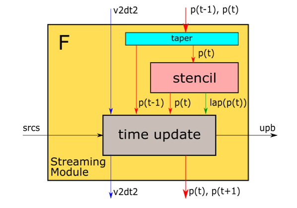
Figure 1. Forward streaming module
Backward streaming module
As shown in Figure 2, the backward function is composed of three modules connected by FIFOs. Two of them labeled with R and S, similar to the forward streaming module, are designed to compute Receiver wavefield and reconstruct Source wavefield respectively. The module labeled with I (Imaging streaming module) realizes Equation (4), whic is used to compute the cross correlation between the two wavefields (Receiver and Source wavefields).
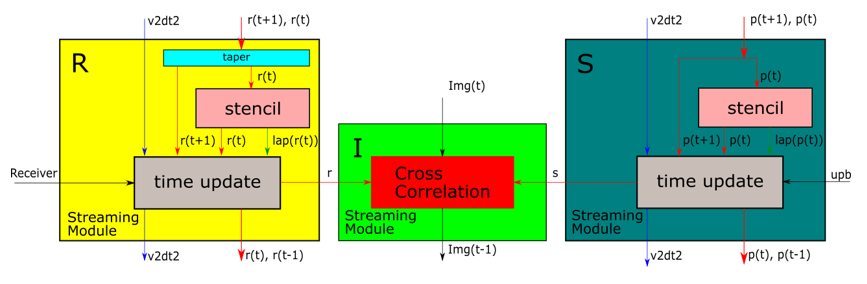
Figure 2. Backward streaming module
3. Stencil3D
Similarly, the template class Stencil3D provides the implementation of Equation (2*) and (3) by function laplacian and function propagate respectly. The laplacian function (also called stencil in Figure 1) applies multiple buffers and shifting registers to achieve high spatial parallism. By assigning values to the template variable t_nPEX and t_nPEZ, the HLS will synthesize a compute IP with the ability to compute the laplacian operation for multiple grid points in one clock cycle. The propagate function (also called time upate in Figure 1) processes multiple data streams in parallel to compute multiple data points of the next wavefield simultaneously.
4. RTM3D
Similarly, template class RTM3D provides the implementation of time step iteration in 3D-RTM. In this class, function forward emulates a single time step in the forward propagation path. There are multiple overload of this function for various boundary conditions e.g. Random Boudnayr Condition (RBC).
The block diagram of forward function given in Figure 1 shows the achieved temporal parallelims, namely computing the wavefield at time step \(t\) and \(t+1\) simultaneouly. The streaming interfaces of the basic modules allow them to be connected directly by FIFOs, which hold the wavefield data without storing them back to external memory. This streamlined architecture is the key to achieve high parallelism both spatially and temporally. Each Forward streaming module labeled with F basically takes the wavefield data from the last time stamp then computes the wavefield for current time stamp and outputs both the data and boundary data to other modules in streams.
| [1] | E.Dussaud,W.W.Symes,P.Williamson,L.Lemaistre,P.Singer, B. Denel, and A. Cherrett, “Computational strategies for reversetime migration,” in SEG Technical Program Expanded Abstracts 2008. Society of Exploration Geophysicists, 2008, pp. 2267– 2271. |
| [2] |
|