Portfolio Optimisation
Caveat
This is not a theoretical description of Portfolio Theory. It simply describes an overview of the maths used in the solution. There are many books and references online that describe the maths and the theory in more detail.
Overview
A Portfolio consists of a holding in a number of risky assets (shares or funds) and optionally a risk free asset (bonds).
Portfolio Optimisation seeks to select the best asset distribution according to an objective. The objective is assumed to be maximizing the return for a given amount of risk (or minimizing the risk for a given required return). The asset risk is quantified by the variance of the asset. This is basically Modern Portfolio Theory or the Markowitz Model.
The starting point for Portfolio Optimisation is a list of daily prices of the available assets.
The daily returns are calculated as: \(\frac{price_n-price_{n-1}}{price_{n-1}}\)
The excess returns are calculated as: \(excess_n = r_n - average\, return\, for\, the\, asset\)
The covariance matrix \(\boldsymbol{\Sigma}\) of the excess returns matrix is calculated as:
\(\boldsymbol{\Sigma} = [\sigma_{ij}] = \frac{\boldsymbol{A^TA}}{M-1}\)
Where \(\boldsymbol{A} =\) excess return matrix \(= \begin{bmatrix} r_{11}-\overline{r_1} & ... & r_{N1}-\overline{r_N} \\ r_{12}-\overline{r_1} & ... & r_{N2}-\overline{r_N} \\ \wr & ... \wr \\ r_{1M}-\overline{r_1} & ... & r_{NM}-\overline{r_N}\end{bmatrix}\)
\(\boldsymbol{A^T}\) is the transpose of \(\boldsymbol{A}\)
\(\overline{r_i}\) is the mean return for asset \(i\)
\(r_{ij}\) is the \(j^{th}\) excess return for asset \(i\)
\(N\) is the number of assets
\(M\) is the number of returns
Global Minimum Variance Portfolio
The Global Minimum Variance Portfolio is the asset weight distribution that minimizes the variance (risk) of the overall portfolio. It can be calculated as: \(\boldsymbol{A_mz_m = b}\)
Where \(A_m\) is \(= \begin{bmatrix} 2\boldsymbol{\Sigma} & \boldsymbol{1} \\ \boldsymbol{1^t} & 0\end{bmatrix}\)
\(\boldsymbol{\Sigma}\) is the covariance matrix, \(\boldsymbol{1}\) is an all one’s vector and \(\boldsymbol{1^t}\) its transpose.
\(\boldsymbol{z_m}\) is the asset weights (plus a Lagrange Multiplier).
\(\boldsymbol{b}\) is a zero vector with the last entry a one.
This equation is solved for \(\boldsymbol{z_m}\) using LU decomposition and back substitution.
Expected Portfolio Return is calculated as: \(\boldsymbol{W^t.\mu}\)
Where \(\boldsymbol{W^t}\) is the transpose of the GMVP weights vector and \(\boldsymbol{\mu}\) is the asset mean returns vector.
Portfolio Variance is calculated as \(\boldsymbol{W^t.\Sigma.W}\)
Efficient Portfolio
An efficient portfolio is the asset weight distribution that minimises the variance (risk) of the overall portfolio given a required target return. It can be calculated as: \(\boldsymbol{A_mz_m = b}\)
Where \(\boldsymbol{A_m}\) is \(\begin{bmatrix} 2\boldsymbol{\Sigma} & \boldsymbol{\mu} & \boldsymbol{1} \\ \boldsymbol{\mu^t} & 0 & 0 \\ \boldsymbol{1^t} & 0 & 0\end{bmatrix}\)
\(\boldsymbol{\Sigma}\) is the covariance matrix, \(\boldsymbol{1}\) is an all one’s vector and \(\boldsymbol{1^t}\) its transpose.
\(\boldsymbol{\mu}\) is the asset mean returns vector and \(\boldsymbol{\mu^t}\) its transpose.
\(\boldsymbol{z_m}\) is the asset weights (plus two Lagrange Multipliers).
\(\boldsymbol{b}\) is a zero vector with the second last entry the portfolio target return and the last entry a one.
This equation is sloved for \(\boldsymbol{z_m}\) using LU decomposition and back substitution.
Tangency Portfolio
Portfolios can be visualized on a graph where the x-axis is risk (portfolio variance) and the y-axis is portfolio return. The efficient frontier is the curve representing the maximum returns for given risks and it’s shape is typically:
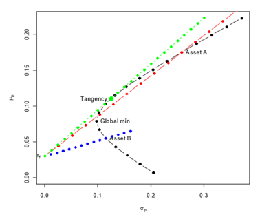
The Tangency Portfolio is the asset weight distribution that maximises the slope (Sharpe Ratio) of a straight line (Capital Market Line) intersecting the the return axis at the risk free rate and passing through the efficient frontier. It can be calculated as: \(\boldsymbol{W_T} = \frac{\boldsymbol{\Sigma^{-1}}(\boldsymbol{\mu}-r_f.\boldsymbol{1})}{\boldsymbol{1^t}\boldsymbol{\Sigma^{-1}}(\boldsymbol{\mu}-r_f.\boldsymbol{1})}\)
Where \(\boldsymbol{W_T}\) is the tangency weights vector
\(\boldsymbol{\Sigma^{-1}}\) is the inverse of the covariance matrix \(\boldsymbol{\Sigma}\)
\(\boldsymbol{\mu}\) is the asset mean returns vector
\(\boldsymbol{1}\) is the all ones vector and \(\boldsymbol{1^t}\) its transpose
\(r_f\) is the risk free rate
This is solved using LU decomposition with back and forward substitution:
\(\boldsymbol{\Sigma^{-1}}(\boldsymbol{\mu}-r_f.\boldsymbol{1}) = Y\)
\((\boldsymbol{\mu}-r_f.\boldsymbol{1}) = Y\boldsymbol{\Sigma}\)
The Sharpe Ratio \(= \frac{Tangency\, expected\, return - r_f}{Tangency\, Standard\, Deviation}\)
Efficient Portfolio of Risky and Risk Free Assets
This is the asset and risk free weight distribution that minimises portfolio risk given a risk free rate and a target portfolio return.
The total wealth is split between the tangency portfolio and the risk free asset.
It is calculated as:
\(Tangency\, Weight = \frac{Target\, return - r_f}{Expected\, return - r_f}\)
And \(Asset\, Weights = Tangency\, Weight.x_T\) where \(x_T\) is the Tangency Portfolio weights vector
And \(Risk\, Free\, Weight = 1 - Tangency\, Weight\)