Black-Scholes Model¶

Overview¶

The Black-Scholes Model is a mathematical model for the dynamics of a financial market containing derivative investment instruments (from wikipedia).

This section explains the stochastic differential equation (stock price process) in continue form and in discrete form (used as stock price process). They are core part for option pricing.

Black-Scholes Model¶

The Continue form of Black-Scholes is:

\[dS_t = \mu S_t dt + \sigma S_t dz\]

where \(S_t\) is the stock price at time \(t\). \(\mu\) is the stock’s expected rate of return. \(\sigma\) is the volatility of the stock price. The random variable \(z\) follows Wiener process, i.e. \(z\) satisfies the following equation.

The change of \(\Delta z\) during a sample period of time \(\Delta t\) is \(\Delta z = \epsilon \sqrt{\Delta t}\), where \(\epsilon\) has a standardized normal distribution \(\phi(0,1)\).

The value of \(\Delta z\) for any two different short intervals of time, \(\Delta t\), are independent.

It follows that \(\Delta z\) has a normal distribution with the mean of \(0\) and the variance of \(\Delta t\).

The Discrete form of Black-Scholes is:

\[\Delta S_t = \mu S_t \Delta t + \sigma S_t \epsilon \sqrt{\Delta t} => \frac{\Delta S_t}{S_t} = \mu \Delta t + \sigma \epsilon \sqrt{\Delta t}\]

The left side of the equation is the return provided by the stock in a short period of time, \(\Delta t\). The term \(\mu \Delta t\) is the expected value of this return, and the \(\sigma \epsilon \sqrt{\Delta t}\) is the stochastic component of the return. It is easy to see that \(\frac{\Delta S_t}{S_t} \sim \phi (\mu \Delta t, \sigma^2 \Delta t)\), i.e. the mean of \(\frac{\Delta S_t}{S_t}\) is \(\mu \Delta t\) and the variance is \(\sigma^2 \Delta t\).

\(Ito\) lemma and direct corollary¶

Suppose that the value of a variable \(x\) follows the \(Ito\) process

\[dx = a(x,t) dt + b(x,t) dz\]

where \(dz\) is a Wiener process and \(a\) and \(b\) are functions of \(x\) and \(t\). The variable \(x\) has a drift rate of \(a\) and a variance rate of \(b^2\). \(Ito\) lemma shows that a function \(G(x,t)\) follows the process

\[dG = (\frac{\partial G}{\partial x} a + \frac{\partial G}{\partial t} + \frac{1}{2} \frac{\partial^2 G}{\partial x^2} b^2) dt + \frac{\partial G}{\partial x} b dz.\]

Thus \(G\) also follows an \(Ito\) process, with a drift rate of \(\frac{\partial G}{\partial x} a + \frac{\partial G}{\partial t} + \frac{1}{2} \frac{\partial^2 G}{\partial x^2} b^2\) and a variance rate of \((\frac{\partial G}{\partial x} b)^2\).

In stock price process \(a(x,t)=\mu S\) and \(b(x,t)=\sigma S\).

Corollary: lognormal property of \(S\)¶

Let us define \(G = \ln S\). With \(Ito\) lemma, we have

\[dG = (\mu - \frac{\sigma^2}{2}) dt + \sigma dz,\]

using

\[\frac{\partial G}{\partial S} = \frac{1}{S}, \frac{\partial^2 G}{\partial S^2} = -\frac{1}{S^2}, \frac{\partial G}{\partial t} = 0.\]

Thus

\[\ln S_T - \ln S_0 \sim \phi [(\mu-\frac{\sigma^2}{2})T, \sigma^2 T].\]

where \(S_T\) is the stock price at a future time \(T\), \(S_0\) is the stock price at time 0. In other words, \(S_T\) has a lognormal distribution, which can take any value between 0 and \(+\infty\).

Implementation of B-S model¶

The discrete form of process for \(\ln S\) is as:

\[\ln S(t+\Delta t) - \ln S(t) = (\mu - \frac{\sigma^2}{2})\Delta t + \sigma \epsilon \sqrt{\Delta t}\]

Its equivalent form is:

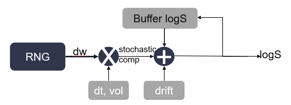
\[S(t+\Delta t) = S(t)\exp [(\mu - \frac{\sigma^2}{2})\Delta t + \sigma \epsilon \sqrt{\Delta t}]\]

The formula above is used to generate the path for \(S\). In order to optimize the multiplication of \(S\) with adder operator in path pricer, in our implementation, the B-S path generator will fetch the normal random number \(\epsilon\) from RNG sequence and output the \(\ln S\) to path pricer.

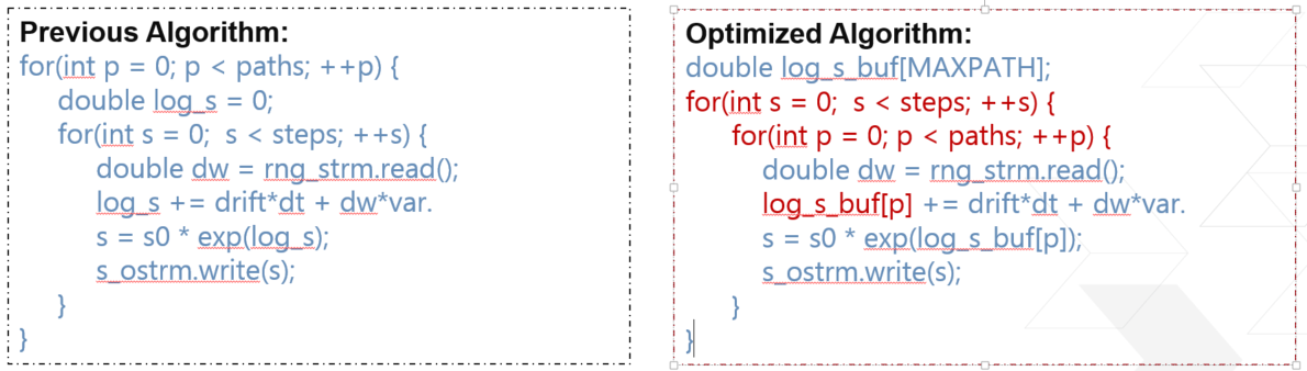
Because there is accumulation of \(\ln S\), the initiation interval (II) cannot achieve 1. Here, change order between paths and steps. Because the input random number are totally independent, the change of order will not affect the accurate of the result. The pseudo-code is shown as follows.