Heston Model
Overview
Heston model is a mathematical model that describing dynamics of underlying asset price. It is a stochastic volatility model which assumes the volatility of the asset price is not constant but follows a random process. In this case, volatility follows square root process which means volatility is always non-negative.
Stochastic Process Equations of the Heston Model
The continuous form of Heston Model is:
Where \(S_t\) is random variable, represent a stock price at time \(t\). \(\mu\) is the stock’s expected rate of return. \(\sqrt[2]{\nu_t}\) is the volatility of stock price and \(\nu_t\) is also a random variable. \(\theta\) is the long term variance. \(\kappa\) is the rate at which \(\nu_t\) revert to \(\theta\). \(\sigma\) is the volatility of the volatility. \(\mathrm{d}W_t^S\) and \(\mathrm{d}W_t^\nu\) are Wiener processes with correlation \(\rho\).
Partial Differential Equation (PED) of Heston Model
In the provided solver, the PDE is the Heston Pricing Model [HESTON1993]. Using the naming conventions of Hout & Foulon [HOUT2010], the PDE is given as:
where:
\(u\) - the price of the European option;
\(s\) - the underlying price of the asset;
\(v\) - the volatility of the underlying price;
\(\sigma\) - the volatility of the volatility;
\(\rho\) - the correlation of Weiner processes;
\(\kappa\) - the mean-reversion rate;
\(\eta\) - the long term mean.
The Heston PDE then describes the evolution of an option price over time (\(t\)) and a solution of this PDE results in the specific option price for an \((s,v)\) pair for a given maturity date \(T\). The finite difference solver maps the \((s,v)\) pair onto a 2D discrete grid, and solves for option price \(u(s,v)\) after \(N\) time-steps.
Implementations
The discrete form (Euler-Maruyama Form) of Heston Model is:
Where \(\Delta\) stands for unit timestep length. \(S(j\Delta)\) stands for S in j th timesteps, AKA \(S(j * \Delta t)\). \(\nu(j\Delta)\) has a similar meaning. To simplify the process, we use \(\ln{S(j\Delta)}\) instead of \(S\) since multiplication becomes addition after logarithm.
\(\Delta W_t^S\) and \(\Delta W_t^\nu\) could be calculated by:
Where \(Z_S\) and \(Z_\nu\) are two uniform distributed random numbers that have correlation \(\rho\)
Although \(\nu\) is non-negative in continuous form, it would become negative if we use the Euler-Maruyama form above directly. There are several variations to solve this issue, here we provide 5 of most commonly used.
kDTReflection: use absolute value of the volatility of the last iteration.
kDTPartialTruncation: use only absolute value of volatility of the last iteration in sqrt root part.
kDTFullTruncation: use only positive part or zero of volatility of the last iteration.
\(\nu((j-1)\Delta)^+ = \nu((j-1)\Delta)\) if \(\nu((j-1)\Delta) > 0\) \(\nu((j-1)\Delta)^+ = 0\) if \(\nu((j-1)\Delta) \leq 0\).
kDTQuadraticExponential and kDTQuadraticExponentialMartingale are more accurate variation, details could be found in reference papers [ANDERSON2005]. They use a different approximation method to calculate \(\nu\), here’s brief on its algorithm
Step 1: we calculate first order moment and second order moment of \(\nu\).
Step 2: Calculate \(\Psi = s^2 / m^2\)
Step 3: If \(\Psi \leq \Psi_{sw}, \Psi_{sw} = 1.5\), Then
Step 3.1: Calculate \(a\) and \(b^2\)
Step 3.2: Calculate \(\nu(j\Delta)\)
Step 4: If Step 3 does not hold, Then
Step 4.1: Calculate \(\beta\) and \(p\)
Step 4.2: Calculate \(U_\nu = \Psi(Z_\nu)\)
Step 4.3: Calculate \(\nu(j\Delta)\)
It should be noticed that they both have two branches for value in different range. These two branches have a similar calculation process. Furthermore, only one branch is active at the same time. By merging these two branches into one branch and manually binding calculations to DSPs, it will cut off DSP cost. This won’t change its performance and accuracy.
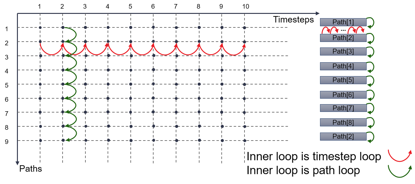
In Monte Carlo Simulation, we need to compute stock prices of multiple paths at multiple time steps. Therefore we need two loops to calculate prices and volatilities, the inner loop is either timestep loop or path loop. Price at each time step is calculated using last time step’s price and volatility as input. And we use 1-D array to store price and volatility of each path’s history (last timestep).
If the inner loop is timestep loop, as red arrows demonstrate in the diagram below, it will keep update the same array element until reaches max timesteps. Such operation can not achieve initiation interval (II)=1 and will greatly slow down the calculation process. If the inner loop is path loop, as green arrows demonstrate in the diagram below, it will keep updating different array element each time. Such operation will avoid dependency issue and reach II=1, which is used in this implementation.
References
| [HESTON1993] | Heston, “A closed-form solution for options with stochastic volatility with applications to bond and currency options”, Rev. Finan. Stud. Vol. 6 (1993) |
| [HOUT2010] | Hout and Foulon, “ADI Finite Difference Schemes for Option Pricing in the Heston Model with correlation”, International Journal of Numerical Analysis and Modeling, Vol 7, Number 2 (2010). |
| [ANDERSON2005] | Anderson, L, “Efficient Simulation of the Heston Stochastic Volatility Model”, (2005). |