Singular Value Decomposition for general matrix (GESVJ)

Overview

One-sided Jacobi alogirhm is a classic and robust method to calculate Singular Value Decompositon (SVD), which can be applied for any dense matrix with the size of $M \times N$. In this library, it is denoted as GESVJ, same as the API name used in LAPACK.

$$A = U \Sigma V^T$$

where $A$ is a dense symmetric matrix of size $m \times n$, $U$ is $m \times m$ matrix with orthonormal columns and and $V$ is $n \times n$ matrix with orthonormal columns, and $\Sigma$ is diagonal matrix. The maximum matrix size supported in FPGA is templated by NRMAX, NCMAX.

Algorithm

The calculation process of one-sided Jacobi SVD method is as follows:

1. Initialize matrix V = I
2. Select two columns (i, j), i < j, of matrix A, namely $A_i$ and $A_j$. Accumulate two columns of data by fomular

$$\begin{split}&b_{ii} = A_i^TA_i = ||A_i||^2 \\ &b_{jj} = A_j^TA_j = ||A_j||^2 \\ &b_{ij} = A_i^TA_j\end{split}$$

A $2 \times 2$ matrix can be obtained and noted as:

$$\begin{split}\begin{bmatrix} b_{ii}\ b_{ij}\\ b_{ji}\ b_{jj}\\ \end{bmatrix}\end{split}$$

where $b_{ij}$ equals $b_{ji}$.

3. Solve the $2 \times 2$ symmetric SVD with Jacobi rotation:

$$\begin{split}&\tau = (b_{ii} - b_{jj}) / (2 * b_{ij})) \\ &t = sign(\tau)/(|\tau| + \sqrt{(1 + \tau^2)}) \\ &c = 1 / \sqrt{(1+t^2)} \\ &s = c * t \\\end{split}$$

if we put s and c in a matrix as J, then J equals

$$\begin{split}\begin{bmatrix} 1\ \ \ \ \ 0\ ...\ 0\ \ 0\ \\ 0\ \ \ \ \ c\ ...\ s\ \ 0\ \\ 0\ \ \ \ \ 0\ ...\ 0\ \ 0\ \\ 0\ -s\ ...\ c\ \ 0\ \\ 0\ \ \ \ \ 0\ ...\ 0\ \ 1\ \\ \end{bmatrix}\end{split}$$

4. Update the i and j columns of matrix A and V by

$$\begin{split}A = A J\\ V = V J\end{split}$$

5. Calculate converage of $2 \times 2$ matrix by

$$conv = |b_{ij}| / \sqrt{(b_{ii}b_{jj})}$$

and select the max converage of all pairs (i, j).

6. Repeat steps 2-4 until all pairs of (i, j) are calculated and updated.
7. If the max converage among all paris of (i, j) is bigger than 1.e-8, repeat steps 2-6 again, which is also called one sweep.
8. When the converge is small enough, calculate the matrix U and S for each $i = 1, ..., n$ by

$$\begin{split}&s_i =||a_i||_2 \\ &u_i = a_i / s_i\end{split}$$

Architecture

From the algorithm, we know that the core part of the computation is two columns of data read-and-accumulate, and then updating corresponding two columns of data in Matrix A and V. In this library, we implement this core module in the following architecture.

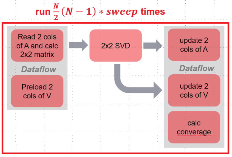
It can be seen from the architecture, steps 2-5 (each pair of i and j) of the algorithm is divided into three stages:

Stage 1:

1. read two columns of data of A to BRAM and accumulate to $b_{ii}$, $b_{jj}$ and $b_{ij}$.
2. preload two columns of data of matrix V to BRAM.

Stage 2:

Calculate SVD for $2 \times 2$ matrix

Stage 3:

1. Update two columns of data in matrix A
2. Update two columns of data in matrix V.
3. Meanwhile, calculate converage for current pair (i, j).

Since operating data of matrix A and V are independent, two modules of stage 1 are running in parallel. Meanwhile, thress modules of stage 3 run in parallel. The last module of stage 3 calculates converage using $2 \times 2$ matrix data. This converage computing process is in read-and-accu module of stage 1 according to the algorithm. However, it requires ~60 cycles, which is also a lot after partitioning matrix A by row. Therefore, this calculation process is extracted as a submodule in stage 3.

Note

Why updating matrix V is divided into two modules?

From the figure, we can see that there are two modules related to matrix V, preload two columns of data of V to BRAM, and updating V. In our design, matrix A and V are all saved in URAM. And for each URAM, only 2 ports of read/write are supported. Since matrix A cummulated $2 \times 2$ data need 100+ cycles to do SVD. We may preload two columns of V into BRAMs via 2-reading ports of URAM. And using two writting ports when updating data in V.

Besides, in order to speed up the data reading and updating of matrix V data, the matrix V is partitioned by NCU through its row. For each CU, matrix V is read/written using 2 URAM ports.

Note

Supported data size:

The supported maximum size of matrix A that templated by NRMAX and NCMAX is 512. The partitioning number MCU and NCU can support up to 16, respectively.