Improving Performance Lab
Introduction
This lab introduces various techniques and directives which can be used in Vitis HLS to improve design performance. The design under consideration accepts an image in a (custom) RGB format, converts it to the Y’UV color space, applies a filter to the Y’UV image and converts it back to RGB.
Objectives
After completing this lab, you will be able to:
- Add directives in your design
- Understand the effect of INLINE directive
- Improve performance using PIPELINE directive
- Distinguish between DATAFLOW directive and Configuration Command functionality
Steps
Create a Vitis HLS Project from Command Line
Validate your design using terminal. Create a new Vitis HLS project from the terminal.
- Invoke Vitis HLS Command prompt by selecting Start > Xilinx Design Tools > Vitis HLS 2022.2 Command Prompt on Windows machine or open a new terminal window on Linux machine.
-
Change directory to {labs}/lab2.
A self-checking program (yuv_filter_test.c) is provided. Using that we can validate the design. A Makefile is also provided. Using the Makefile, the necessary source files can be compiled and the compiled program can be executed. You can examine the contents of these files and the project directory.
- In the terminal, type make to compile and execute the program. (You might need to set up the system environment variable for make command)
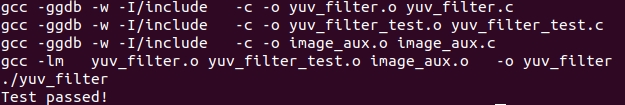
Validating the design
Note that the source files (yuv_filter.c, yuv_filter_test.c, and image_aux.c) were compiled, yuv_filter executable program was created, and then it was executed.
The program tests the design and outputs Test passed message.
A Vitis HLS tcl script file (pynq_yuv_filter.tcl) is provided and can be used to create a Vitis HLS project.
- Type vitis_hls -f pynq_yuv_filter.tcl in the terminal to create the project targeting xc7z020clg400-1 part. The project will be created and the vitis_hls.log file will be generated.
- Open the vitis_hls.log file from {labs}/lab2 using any text editor and observe the following sections:
- Creating directory and project called yuv_filter.prj within it, adding design files to the project, setting solution name as solution1, setting target device, setting desired clock period, and importing the design and testbench files.
- Synthesizing (Generating) the design which involves scheduling and binding of each functions and sub-function.
- Generating RTL of each function and sub-function in Verilog and VHDL languages.
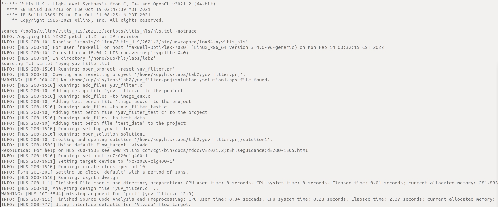
Creating project and setting up parameters
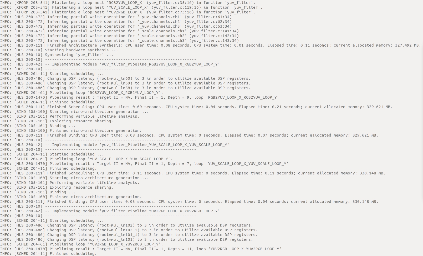
Synthesizing (Generating) the design
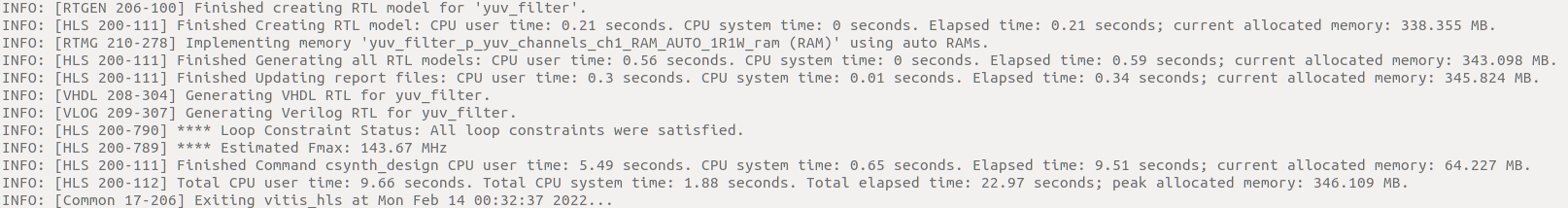
Generating RTL
- Open the created project (in GUI mode) from the terminal, by typing vitis_hls -p yuv_filter.prj. The Vitis HLS will open in GUI mode and the project will be opened.
Analyze the Created Project and Results
Open the source file and note that three functions are used. Look at the results and observe that the latencies are undefined (represented by ?).
- In Vitis HLS GUI, expand the source folder in the Explorer view and double click yuv_filter.c to view the content.
- The design is implemented in 3 functions: rgb2yuv, yuv_scale and yuv2rgb.
- Each of these filter functions iterates over the entire source image (which has maximum dimensions specified in image_aux.h), requiring a single source pixel to produce a pixel in the result image.
- The scale function simply applies individual scale factors, supplied as top-level arguments to the Y’UV components.
- Notice that most of the variables are of user-defined (typedef) and aggregate (e.g. structure, array) types.
- Also notice that the original source used malloc() to dynamically allocate storage for the internal image buffers. While appropriate for such large data structures in software, malloc() is not synthesizable and is not supported by Vitis HLS.
- A viable workaround is conditionally compiled into the code, leveraging the SYNTHESIS macro. Vitis HLS automatically defines the SYNTHESIS macro when reading any code. This ensure the original malloc() code is used outside of synthesis but Vitis HLS will use the workaround when synthesizing.
- Expand the syn > report folder in the Explorer view and double-click yuv_filter_csynh.rpt entry to open the synthesis report.
- Each of the loops in this design has variable bounds – the width and height are defined by members of input type image_t. When variables bounds are present on loops the total latency of the loops cannot be determined: this impacts the ability to perform analysis using reports. Hence, “?” is reported for various latencies.
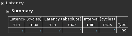
Latency computation
Apply TRIPCOUNT Pragma
Open the source file and uncomment pragma lines, re-synthesize, and observe the resources used as well as estimated latencies. Answer the questions listed in the detailed section of this step.
-
To assist in providing loop-latency estimates, Vitis HLS provides a TRIPCOUNT directive which allows limits on the variables bounds to be specified by the user. In this design, such directives have been embedded in the source code, in the form of #pragma statements.
-
Uncomment the #pragma lines (76, 79, 116, 119, 156, 159) to define the loop bounds and save the file.
- Synthesize the design by selecting Solution > Run C Synthesis > Active Solution. View the synthesis report when the process is completed.
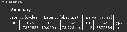
Latency computation after applying TRIPCOUNT pragma
Question 1
Answer the following question pertaining to yuv_filter function.
Estimated clock period:
Worst case latency:
Number of DSP48E used:
Number of BRAMs used:
Number of FFs used:
Number of LUTs used: - Expand the Module & loop and note the latency and trip count numbers for the yuv_scale function. Note that the iteration latency of YUV_SCALE_LOOP_X_YUV_SCALE_LOOP_Y is 6x the specified TRIPCOUNT, implying that 6 cycles are used for each of the iteration of the loop.
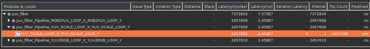
Loop latency
Note that YUV_SCALE_LOOP_X_YUV_SCALE_LOOP_Y is already pipelined. -pipeline_loops
specifies the lower limit used when automatically pipelining loops. The default is 64, causing Vitis HLS to automatically pipeline loops with a tripcount of 64, or greater. If the option is applied, the innermost loop with a tripcount higher than the threshold is pipelined, or if the tripcount of the innermost loop is less than or equal to the threshold, its parent loop is pipelined. If the innermost loop has no parent loop, the innermost loop is pipelined regardless of its tripcount. - You can verify this by opening the Schedule Viewer, and expand the YUV_SCALE_LOOP_X entry.
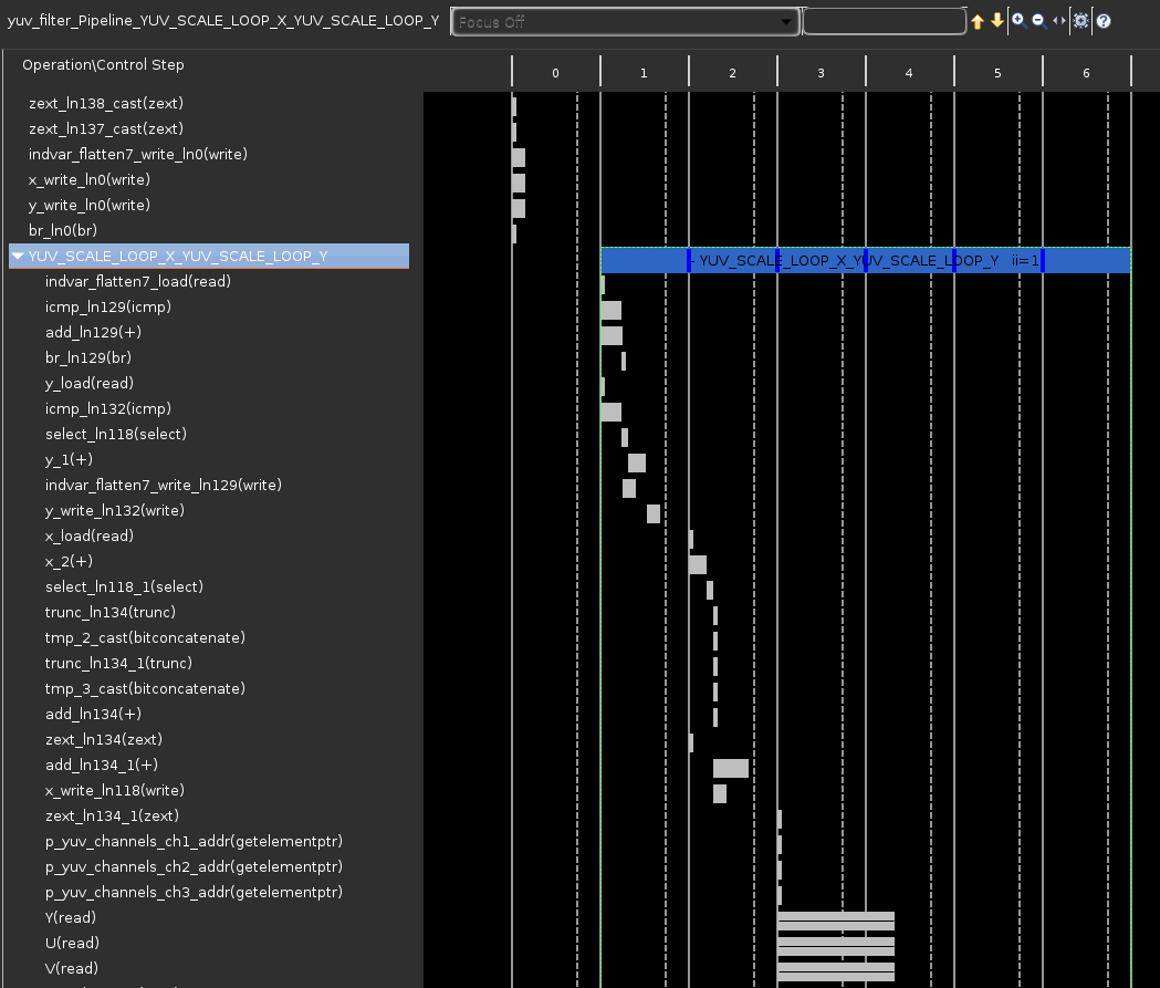
Design analysis view of the YUV_SCALE_LOOP_Y loop
-
In the report tab, expand and click on the yuv_filter_Pipeline_RGB2YUV_LOOP_X_RGB2YUV_LOOP_Y entry to open the report.
Question 2
Answer the following question pertaining to rgb2yuv function.
Estimated clock period:
Worst case latency:
Number of DSP48E used:
Number of FFs used:
Number of LUTs used: -
Similarly, open the yuv2rgb report.
Question 3
Answer the following question pertaining to yuv2rgb function.
Estimated clock period:
Worst case latency:
Number of DSP48E used:
Number of FFs used:
Number of LUTs used:
Remove the pipeline optimization done by Vitis HLS automatically by adding pipeline off pragma
- Select Project > New Solution.
- A Solution Configuration dialog box will appear. Note that the check boxes of Copy directives and constraints from solution are checked with solution1 selected. Click the Finish button to create a new solution with the default settings.
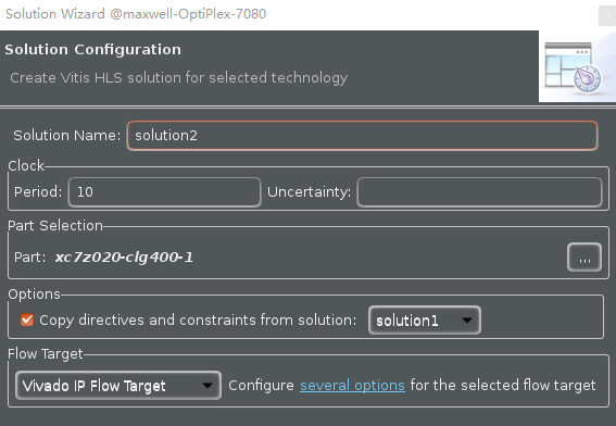
Creating a new Solution after copying the existing solution
- Make sure that the yuv_filter.c source is opened and visible in the information pane, and click on the Directive tab.
- Select function RGB2YUV_LOOP_X in the directives pane, right-click on it, and select Insert Directive…
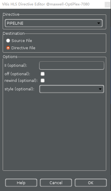
- Click on the drop-down button of the Directive field. A pop-up menu shows up listing various directives. Select PIPELINE directive.
- In the Vitis HLS Directive Editor dialog box, click on the off option to turn off the automatic pipelining. Make sure that the Directive File is selected as destination. Click OK.
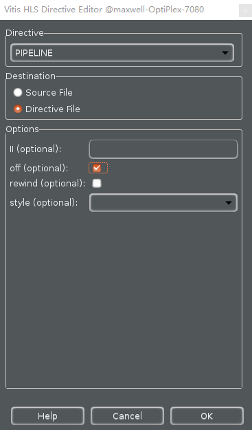
Add PIPELINE off directive
- Similarly, apply the PIPELINE off directive to YUV2RGB_LOOP_X, YUV2RGB_LOOP_Y, YUV_SCALE_LOOP_X, YUV_SCALE_LOOP_Y and RGB2YUV_LOOP_Y objects. At this point, the Directive tab should look like as follows.
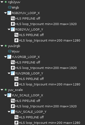
PIPELINE off directive applied
- Click on the Synthesis button.
- When the synthesis is completed, report shows the performance and area without the automatic optimization of Vitis HLS.
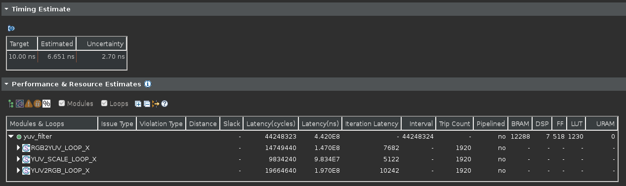
Performance after applying PIPELINE off directive
Apply PIPELINE Directive
Create a new solution by copying the previous solution settings. Apply the PIPELINE directive. Generate the solution and understand the output.
- Select Project > New Solution.
- A Solution Configuration dialog box will appear. Click the Finish button (with copy from Solution2 selected).
- Make sure that the yuv_filter.c source is opened and visible in the information pane, and click on the Directive tab.
- Select the pragma HLS PIPELINE off of RGB2YUV_LOOP_Y in the directives pane, right-click on it, and select Modify Directive
- In the Vitis HLS Directive Editor dialog box, click the off option to turn on the pipelining. Make sure that the Directive File is selected as destination. Click OK.
Add PIPELINE directive
- When an object (function or loop) is pipelined, all the loops below it, down through the hierarchy, will be automatically unrolled.
- In order for a loop to be unrolled it must have fixed bounds: all the loops in this design have variable bounds, defined by an input argument variable to the top-level function.
- Note that the TRIPCOUNT directive on the loops only influences reporting, it does not set bounds for synthesis.
- Neither the top-level function nor any of the sub-functions are pipelined in this example.
- The pipeline directive must be applied to the inner-most loop in each function – the innermost loops have no variable-bounded loops inside which are required to be unrolled and the outer loop will simply keep the inner loop fed with data.
- Leave II (Initiation Interval) blank as Vitis HLS will try for an II=1, one new input every clock cycle.
- Click OK.
- Similarly, apply the PIPELINE directive to YUV2RGB_LOOP_Y and YUV_SCALE_LOOP_Y objects, but remove the PIPELINE directive of YUV2RGB_LOOP_X, YUV_SCALE_LOOP_X and RGB2YUV_LOOP_X. At this point, the Directive tab should look like as follows.
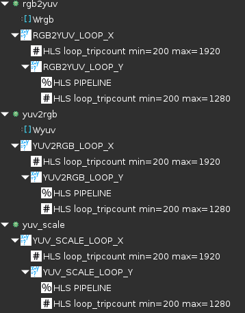
PIPELINE directive applied
- Click on the Synthesis button.
- When the synthesis is completed, select Project > Compare Reports… to compare the two solutions.
- Select Solution2 and Solution3 from the Available Reports, and click on the Add» button.
- Observe that the latency reduced.
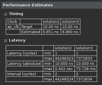
Performance comparison after pipelining
In Solution2, the total loop latency of the inner-most loop was loop_body_latency x loop iteration count, whereas in Solution3 the new total loop latency of the inner-most loop is loop_body_latency + loop iteration count.
- Scroll down in the comparison report to view the resources utilization. Observe that the FFs, LUTs, and DSP48E utilization increased whereas BRAM remained same.
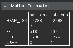
Resources utilization after pipelining
Apply DATAFLOW Directive and Configuration Command
Create a new solution by copying the previous solution (Solution3) settings. Apply DATAFLOW directive. Generate the solution and understand the output.
- Select Project > New Solution.
- A Solution Configuration dialog box will appear. Click the Finish button (with copy from Solution4 selected).
- Close all inactive solution windows by selecting Project > Close Inactive Solution Tabs.
- Make sure that the yuv_filter.c source is opened in the information pane and select the Directive tab.
- Select function yuv_filter in the Directive pane, right-click on it and select Insert Directive…
- A pop-up menu shows up listing various directives. Select DATAFLOW directive and click OK.
- Click on the Synthesis button.
- When the synthesis is completed, the synthesis report is automatically opened.
- Observe additional information, Dataflow Type, in the Performance Estimates section is mentioned.
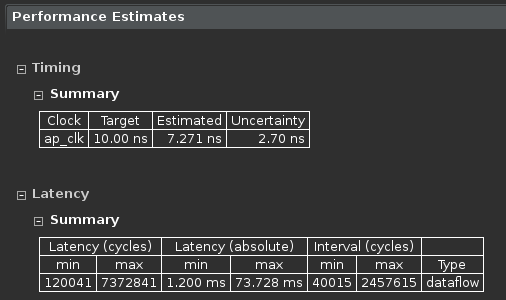
Performance estimate after DATAFLOW directive applied
- The Dataflow pipeline throughput indicates the number of clocks cycles between each set of inputs reads. If this throughput value is less than the design latency it indicates the design can start processing new inputs before the currents input data are output.
- While the overall latencies haven’t changed significantly, the dataflow throughput is showing that the design can achieve close to the theoretical limit (1920x1280 = 2457600) of processing one pixel every clock cycle.
- Scrolling down into the Utilization Estimates section, observe that the number of BRAMs required has doubled. This is due to the default ping-pong buffering in dataflow.
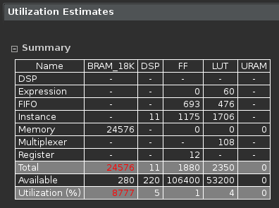
Resource estimate with DATAFLOW directive applied
- When DATAFLOW optimization is performed, memory buffers are automatically inserted between the functions to ensure the next function can begin operation before the previous function has finished. The default memory buffers are ping-pong buffers sized to fully accommodate the largest producer or consumer array.
- Vitis HLS allows the memory buffers to be the default ping-pong buffers or FIFOs. Since this design has data accesses which are fully sequential, FIFOs can be used. Another advantage to using FIFOs is that the size of the FIFOs can be directly controlled (not possible in ping-pong buffers where random accesses are allowed).
- The memory buffers type can be selected using Vitis HLS Configuration command.
Apply Dataflow configuration command, generate the solution, and observe the improved resources utilization.
- Select Solution > Solution Settings… to access the configuration command settings.
- In the Configuration Settings dialog box, expand config_dataflow folder.
- Set fifo as the default_channel. Enter 2 as the fifo_depth. Click OK.
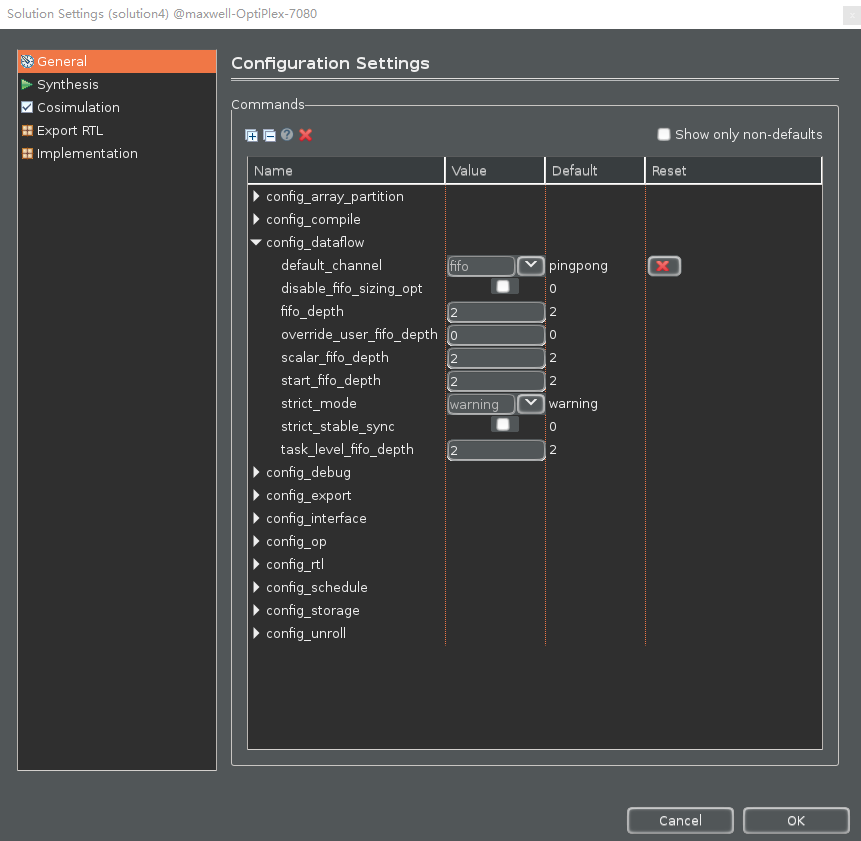
Selecting Dataflow configuration command and FIFO as buffer
- Click OK again.
- Click on the Synthesis button.
- When the synthesis is completed, the synthesis report is automatically opened.
- Note that the latency has reduced. Since this design has data accesses which are fully sequential, the data can flow to next function without waiting all pixels to be processed.
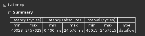
Latency estimation after Dataflow configuration command
Conclusion
In this lab, you learned that even though this design could not be pipelined at the top-level, a strategy of pipelining the individual loops and then using dataflow optimization to make the functions operate in parallel was able to achieve the same high throughput, processing one pixel per clock. When DATAFLOW directive is applied, the default memory buffers (of ping-pong type) are automatically inserted between the functions. Using the fact that the design used only sequential (streaming) data accesses allowed the costly memory buffers associated with dataflow optimization to be replaced with simple 2 element FIFOs using the Dataflow command configuration.
Answers
- Answers for question 1:
Estimated clock period: 6.960 ns
Worst case latency: 7372833
Number of DSP48E used: 8
Number of BRAMs used: 12288
Number of FFs used: 932
Number of LUTs used: 1728 - Answers for question 2:
Estimated clock period: 6.960 ns
Worst case latency: 2457608
Number of DSP48E used: 3
Number of FFs used: 358
Number of LUTs used: 592 - Answers for question 3:
Estimated clock period: 6.960 ns
Worst case latency: 2457610
Number of DSP48E used: 4
Number of FFs used: 255
Number of LUTs used: 423
Copyright© 2022, Advanced Micro Devices, Inc.