Improving Area and Resoudesign.rce Utilization Lab
Introduction
This lab introduces various techniques and directives which can be used in Vitis HLS to improve design performance as well as area and resource utilization. The design under consideration performs Discrete Cosine Transformation (DCT) on an 8x8 block of data.
This design implements a discrete cosine transformation (DCT), and it is provided as C source. The function leverages a 2D DCT algorithm by first processing each row of the input array via a 1D DCT, then processing the columns of the resulting array through the same 1D DCT. It calls the read_data, dct_2d, and write_data functions.
Objectives
After completing this lab, you will be able to:
- Add directives in your design
- Improve performance using PIPELINE directive
- Distinguish between DATAFLOW directive and Configuration Command functionality
- Apply memory partitions techniques to improve resource utilization
Steps
Validate the Design from Command Line
Validate your design in the terminal.
- Open a terminal.
- Change directory to {labs}/lab3.
A self-checking program (dct_test.c) is provided. Using that we can validate the design. A Makefile is also provided. Using the Makefile, the necessary source files can be compiled and the compiled program can be executed.
- Invoke Vitis HLS Command prompt by selecting Start > Xilinx Design Tools > Vitis HLS 2021.2 Command Prompt. In the terminal, type make to compile and execute the program.
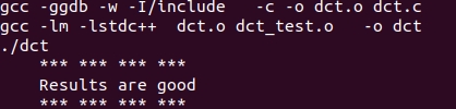
Validating the design
Note that the source files (dct.c and dct_test.c are compiled, then dct executable program was created, and then it was executed. The program tests the design and outputs Results are good message.
Create a New Project
Create a new project in Vitis HLS GUI targeting xc7z020clg400-1.
- Type vitis_hls in the terminal.
- In the Vitis HLS GUI, click on Create Project. The New Vitis HLS Project wizard opens.
- Click Browse… button of the Location field and browse to {labs}/lab3 and then click OK.
- For Project Name, type dct and click Next.
- In the Add/Remove Files for the source files, type dct as the top function name (the provided source file contains the function, to be synthesized, called dct).
- Click the Add Files… button, select dct.c file from the {labs}/lab3 folder, and then click Open.
- Click Next.
- In the Add/Remove Testbench Files for the testbench, click the Add Files… button, select dct_test.c, in.dat, out.golden.dat files from the {labs}/lab3 folder and click Open.
- Click Next.
- In the Solution Configuration page, leave Solution Name field as solution1 and set the clock period as 10. Leave Uncertainty field blank.
- Click on Part’s Browse button, and select the following filters, using the Parts Specify option, to select xc7z020clg400-1.
- Click Finish.
- Double-click on the dct.c under the source folder to open its content in the information pane.
The design under consideration
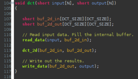
The top-level function dct, is defined at line 104. It implements 2D DCT algorithm by first processing each row of the input array via a 1D DCT then processing the columns of the resulting array through the same 1D DCT. It calls read_data, dct_2d, and write_data functions. The read_data function is defined at line 80 and consists of two loops – RD_Loop_Row and RD_Loop_Col. The write_data function is defined at line 92 and consists of two loops to perform writing the result. The dct_2d function, defined at line 49, calls dct_1d function and performs transpose. Finally, dct_1d function, defined at line 30, uses dct_coeff_table and performs the required function by implementing a basic iterative form of the 1D Type-II DCT algorithm. Following figure shows the function hierarchy on the left-hand side, the loops in the order they are executes and the flow of data on the right-hand side.
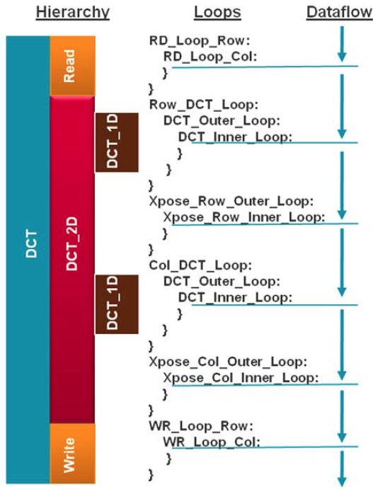
Design hierarchy and dataflow
Synthesize the Design
Synthesize the design with the defaults. View the synthesis results and answer the question listed in the detailed section of this step.
- Select Solution > Run C Synthesis > Active Solution to start the synthesis process.
-
When synthesis is completed, several report files will become accessible and the Synthesis Results will be displayed in the information pane.
The dct_1d, dct_2d, read_data and write_data functions are inlined. Verify this by scrolling up into the Vitis HLS Console view.
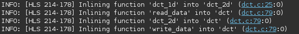
Inlining of dct_1d, dct_2d, read_data and write_data functions
- The Synthesis Report shows the performance and resource estimates as well as estimated latency in the design. Note that the design is already pipelined.
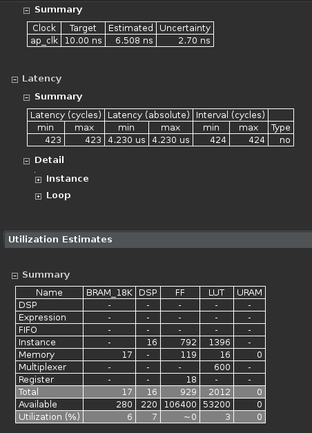
Synthesis report
-
Using scroll bar on the right, scroll down into the report and answer the following question.
Question 1
Answer the following question:
Estimated clock period:
Worst case latency:
Number of DSP48E used:
Number of BRAMs used:
Number of FFs used:
Number of LUTs used: - The report also shows the top-level interface signals generated by the tools.
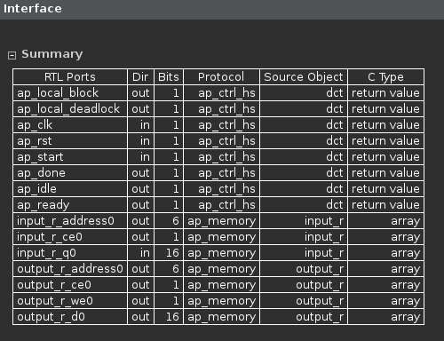
Generated interface signals
You can see ap_clk, ap_rst are automatically added. The ap_start, ap_done, ap_idle, and ap_ready are top-level signals used as handshaking signals to indicate when the design is able to accept next computation command (ap_idle), when the next computation is started (ap_start), and when the computation is completed (ap_done). The top-level function has input and output arrays, hence an ap_memory interface is generated for each of them.
Run Co-Simulation
Run the Co-simulation, selecting Verilog. Verify that the simulation passes.
-
Select Solution > Run C/RTL Co-simulation to open the dialog box so the desired simulations can be run. A C/RTL Co-simulation Dialog box will open.
-
Select the Verilog option, and click OK to run the Verilog simulation using Vivado XSIM simulator.
The RTL Co-simulation will run, generating and compiling several files, and then simulating the design. In the console window you can see the progress and also a message that the test is passed.
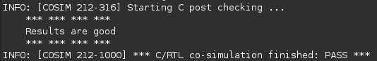
RTL Co-Simulation results
Remove the pipeline optimization done by Vitis HLS automatically by adding pipeline off pragma
- Select Project > New Solution.
- A Solution Configuration dialog box will appear. Note that the check boxes of Copy directives and constraints from solution are checked with solution1 selected. Click the Finish button to create a new solution with the default settings.
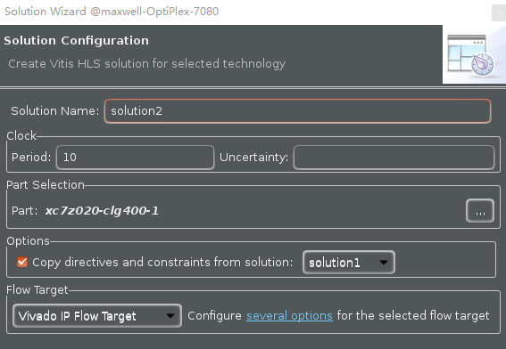
Creating a new Solution after copying the existing solution
- Make sure that the dct.c source is opened and visible in the information pane, and click on the Directive tab.
- Select function DCT_Inner_Loop in the directives pane, right-click on it, and select Insert Directive…
- Click on the drop-down button of the Directive field. A pop-up menu shows up listing various directives. Select PIPELINE directive.
- In the Vitis HLS Directive Editor dialog box, click on the off option to turn off the automatic pipelining. Make sure that the Directive File is selected as destination. Click OK.
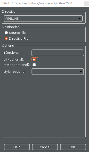
Add PIPELINE off directive
- Similarly, apply the PIPELINE off directive to DCT_Outer_Loop, Row_DCT_Loop, Xpose_Row_Outer_Loop, Xpose_Row_Inner_Loop, Col_DCT_Loop, Xpose_Col_Outer_Loop, Xpose_Col_Inner_Loop, RD_Loop_Row, RD_Loop_Col, WR_Loop_Row, and WR_Loop_Col objects. At this point, the Directive tab should look like as follows.
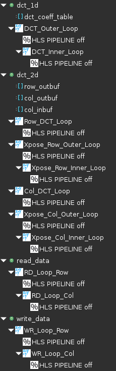
PIPELINE off directive applied
- Click on the Synthesis button.
- When the synthesis is completed, report shows the performance and area without the automatic optimization of Vitis HLS.
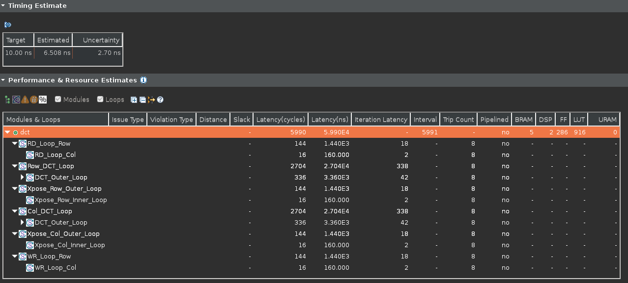
Performance after applying PIPELINE off directive
Apply PIPELINE Directive
Create a new solution by copying the previous solution settings. Apply the PIPELINE directive to DCT_Inner_Loop, Xpose_Row_Inner_Loop, Xpose_Col_Inner_Loop, RD_Loop_Col, and WR_Loop_Col. Generate the solution and analyze the output.
- Select Project > New Solution.
- A Solution Configuration dialog box will appear. Click the Finish button (with copy from Solution2 selected).
- Make sure that the dct.c source is opened in the information pane and click on the Directive tab.
- Select the pragma HLS PIPELINE off of DCT_Inner_Loop of the dct_1d function in the Directive pane, right-click on it and select Modify Directive
- In the Vitis HLS Directive Editor dialog box, click the off option to turn on the pipelining. Make sure that the Directive File is selected as destination. Click OK.
- Leave II (Initiation Interval) blank as Vitis HLS will try for an II=1, one new input every clock cycle.
- Click OK.
- Similarly, apply the PIPELINE directive to Xpose_Row_Inner_Loop and Xpose_Col_Inner_Loop of the dct_2d function, and RD_Loop_Col of the read_data function, and WR_Loop_Col of the write_data function. But remove the PIPELINE directive of DCT_Outer_Loop, Row_DCT_Loop, Xpose_Row_Outer_Loop, Col_DCT_Loop, Xpose_Col_Outer_Loop, RD_Loop_Row and WR_Loop_Row. At this point, the Directive tab should look like as follows.
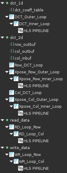
PIPELINE directive applied
- Click on the Synthesis button.
- When the synthesis is completed, select Project > Compare Reports… to compare the two solutions.
- Select Solution2 and Solution3 from the Available Reports, click on the Add» button, and then click OK.
- Observe that the latency reduced from 5990 to 2451 clock cycles.
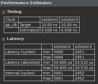
Performance comparison after pipelining
- Scroll down in the comparison report to view the resources utilization. Observe that the FFs and/or LUTs utilization increased whereas BRAM and DSP48E remained same.
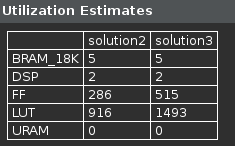
Resources utilization after pipelining
Open the Schedule Viewer and determine where most of the clock cycles are spend, i.e. where the large latencies are.
- Click on the Solution > Open Schedule Viewer .
- Select the dct entry and observe the RD_Loop_Row_RD_Loop_Col and WR_Loop_Row_WR_Loop_Col entries in the Performance & Resource Estimates. These are two nested loops flattened and given the new names formed by appending inner loop name to the outer loop name. You can verify this by looking in the Console view message.
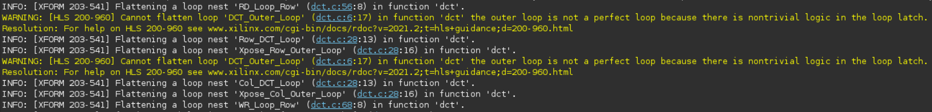
The console view content indicating loops flattening
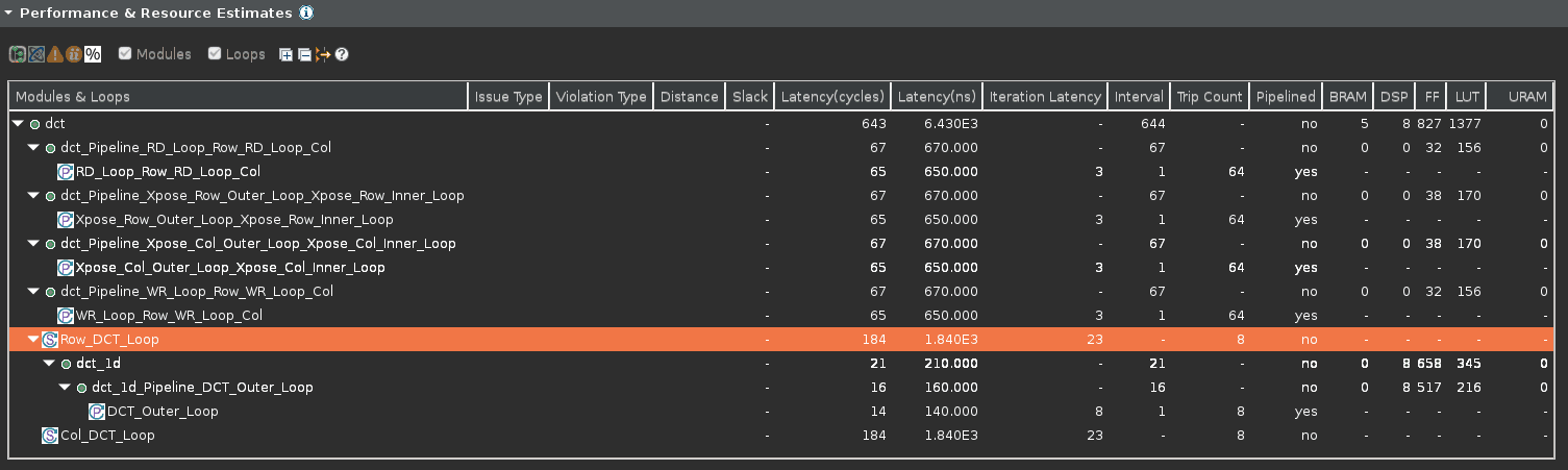
- In the Performance & Resource Estimates pane, expand all items. Notice that the most of the latency occurs is in Row_DCT_Loop_DCT_Outer_Loop and Col_DCT_Loop_DCT_Outer_Loop function.
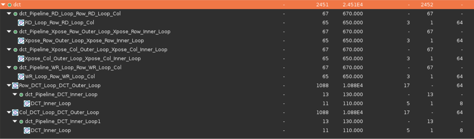
The Performance & Resource Estimates of dct
- In the Schedule Viewer pane, select the Col_DCT_Loop_DCT_Outer_Loop entry, right-click on the col_outbuf_addr_write_In19 (write) block in the Schedule Viewer, and select Goto Source. Notice that line 45 is highlighted which is preventing the flattening of the DCT_Outer_Loop.
Understanding what is preventing DCT_Outer_Loop flattening
- Switch to the Synthesis perspective.
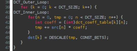
Create a new solution by copying the previous solution settings. Apply fine-grain parallelism of performing multiply and add operations of the inner loop of dct_1d using PIPELINE directive by moving the PIPELINE directive from inner loop to the outer loop of dct_1d. Generate the solution and analyze the output.
- Select Project > New Solution.
- A Solution Configuration dialog box will appear. Click the Finish button (with Solution3 selected).
- Select PIPELINE directive of DCT_Inner_Loop of the dct_1d function in the Directive pane, right-click on it and select Remove Directive.
- Select DCT_Outer_Loop of the dct_1d function in the Directive pane, right-click on it and select Insert Directive…
- A pop-up menu shows up listing various directives. Select PIPELINE directive.
- Click OK.
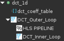
PIPELINE directive applied to DCT_Outer_Loop
By pipelining an outer loop, all inner loops will be unrolled automatically (if legal), so there is no need to explicitly apply an UNROLL directive to DCT_Inner_Loop. Simply move the pipeline to the outer loop: the nested loop will still be pipelined but the operations in the inner-loop body will operate concurrently.
- Click on the Synthesis button.
- When the synthesis is completed, select Project > Compare Reports… to compare the two solutions.
- Select Solution3 and Solution4 from the Available Reports, click on the Add» button, and then click OK.
- Observe that the latency reduced from 2451 to 643 clock cycles.
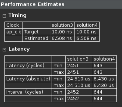
Performance comparison after pipelining
- Scroll down in the comparison report to view the resources utilization. Observe that the utilization of DSP and FF increased. Since the DCT_Inner_Loop was unrolled, the parallel computation requires 8 DSP48E.
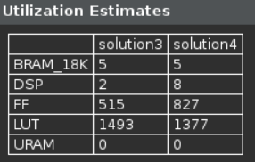
Resources utilization after pipelining
Perform design analysis and look at the dct performance view.
- Switch to the Performance & Resource Estimates in Synthesis Summary.
- Expand, if necessary, and notice that the DCT_Outer_Loop is now pipelined and there is no DCT_Inner_Loop entry.
DCT_Outer_Loop flattening
Improve Memory Bandwidth
Create a new solution by copying the previous solution (Solution3) settings. Apply ARRAY_PARTITION directive to buf_2d_in of dct (since the bottleneck was on src port of the dct_1d function, which was passed via in_block of the dct_2d function, which in turn was passed via buf_2d_in of the dct function) and col_inbuf of dct_2d. Generate the solution.
- Select Project > New Solution to create a new solution.
- A Solution Configuration dialog box will appear. Click the Finish button (with Solution4 selected).
-
With dct.c open, select buf_2d_in array of the dct function in the Directive pane, right-click on it and select Insert Directive…
The buf_2d_in array is selected since the bottleneck was on src port of the dct_1d function, which was passed via in_block of the dct_2d function, which in turn was passed via buf_2d_in of the dct function).
- A pop-up menu shows up listing various directives. Select ARRAY_PARTITION directive.
- Make sure that the type is complete. Enter 2 in the dimension field and click OK.
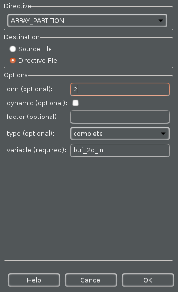
Applying ARRAY_PARTITION directive to memory buffer
- Similarly, apply the ARRAY_PARTITION directive with dimension of 2 to the col_inbuf array.
- Click on the Synthesis button.
- When the synthesis is completed, select Project > Compare Reports… to compare the two solutions.
- Select Solution4 and Solution5 from the Available Reports, and click on the Add» button.
- Observe that the latency reduced from 643 to 579 clock cycles.
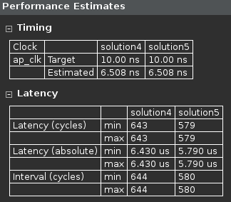
Performance comparison after array partitioning
- Scroll down in the comparison report to view the resources utilization. Observe the increase in the FF resource utilization (almost double).
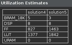
Resources utilization after array partitioning
- Expand the Loop entry in the Performance & Resource Estimates in Synthesis Summary and observe that the Pipeline II is now 1.
Apply DATAFLOW Directive
Create a new solution by copying the previous solution (Solution5) settings. Apply the DATAFLOW directive to improve the throughput. Generate the solution and analyze the output.
- Select Project > New Solution.
- A Solution Configuration dialog box will appear. Click the Finish button (with Solution5 selected).
- Close all inactive solution windows by selecting Project > Close Inactive Solution Tabs.
- Select function dct in the directives pane, right-click on it and select Insert Directive…
- Select DATAFLOW directive to improve the throughput.
- Click on the Synthesis button.
- When the synthesis is completed, the synthesis report is automatically opened.
- Observe that dataflow type pipeline throughput is listed in the “Performance Estimates*
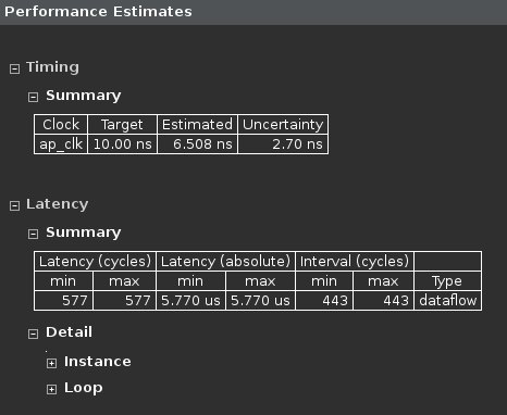
Performance estimate after DATAFLOW directive applied
- The Dataflow pipeline throughput indicates the number of clock cycles between each set of inputs reads (interval parameter). If this value is less than the design latency it indicates the design can start processing new inputs before the currents input data are output.
- Note that the dataflow is only supported for the functions and loops at the top-level, not those
which are down through the design hierarchy. Only loops and functions exposed at the toplevel
of the design will get benefit from dataflow optimization.
- Scrolling down into the Utilization Estimates, observe that the number of BRAM_18K required at the top-level remained at 3.
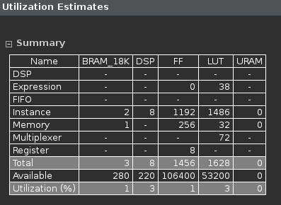
Resource estimate with DATAFLOW directive applied
- Look at the console view and notice that dct_coeff_table is automatically partitioned in dimension 2.
- The buf_2d_in and col_inbuf arrays are partitioned as we had applied the directive in the previous run. The dataflow is applied at the top-level which created channels between top-level functions read_data, dct_2d, and write_data.
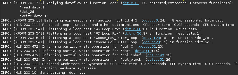
Console view of synthesis process after DATAFLOW directive applied
Perform performance analysis by switching to the Synthesis Summary and looking at the dct Performance & Resource Estimates view.
- Switch to the Synthesis Summary perspective, expand the Performance & Resource Estimates entries, and select the dct_2d entry.
- Observe that most of the latency and interval (throughput) is caused by the dct_2d function. The interval of the top-level function dct, is less than the sum of the intervals of the read_data, dct_2d, and write_data functions indicating that they operate in parallel and dct_2d is the limiting factor. It can be seen that dct_2d is not completely operating in parallel as Row_DCT_Loop and Col_DCT_Loop were not pipelined.
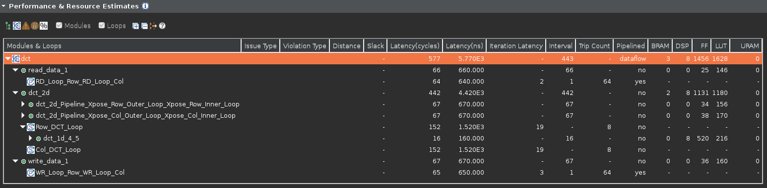
Performance analysis after the DATAFLOW directive
One of the limitations of the dataflow optimization is that it only works on top-level loops and functions. One way to have the blocks in dct_2d operate in parallel would be to pipeline the entire function. This however would unroll all the loops and can sometimes lead to a large area increase. An alternative is to raise these loops up to the top-level of hierarchy, where dataflow optimization can be applied, by removing the dct_2d hierarchy, i.e. inline the dct_2d function.
Apply INLINE Directive
Create a new solution by copying the previous solution (Solution6) settings. Apply INLINE directive to dct_2d. Generate the solution and analyze the output.
- Select Project > New Solution.
- A Solution Configuration dialog box will appear. Click the Finish button (with Solution6 selected).
- Select the function dct_2d in the directives pane, right-click on it and select Insert Directive…
- A pop-up menu shows up listing various directives. Select INLINE directive. The INLINE directive causes the function to which it is applied to be inlined: its hierarchy is dissolved.
- Click on the Synthesis button.
- When the synthesis is completed, the synthesis report will be opened.
- Observe that the latency reduced from 577 to 416 clock cycles, and the Dataflow pipeline throughput drastically reduced from 443 to 73 clock cycles.
- Examine the synthesis log to see what transformations were applied automatically.
- The dct_1d function calls are now automatically inlined into the loops from which they are called, which allows the loop nesting to be flattened automatically.
- Note also that the DSP48E usage has doubled (from 8 to 16). This is because, previously a single instance of dct_1d was used to do both row and column processing; now that the row and column loops are executing concurrently, this can no longer be the case and two copies of dct_1d are required: Vitis HLS will seek to minimize the number of clocks, even if it means increasing the area.
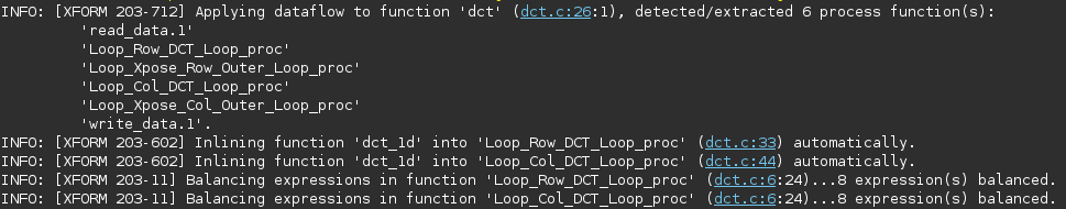
Console view after INLINE directive applied to dct_2d
-
Switch to the Synthesis Summary perspective, expand the Performance & Resource Estimates entries, and select the dct entry.
Observe that the dct_2d entry is now replaced with dct_Loop_Row_DCT_Loop_proc, dct_Loop_Xpose_Row_Outer_Loop_proc, dct_Loop_Col_DCT_Loop_proc, and dct_Loop_Xpose_Col_Outer_Loop_proc since the dct_2d function is inlined. Also observe that all the functions are operating in parallel, yielding the top-level function interval (throughput) of 73 clock cycles.
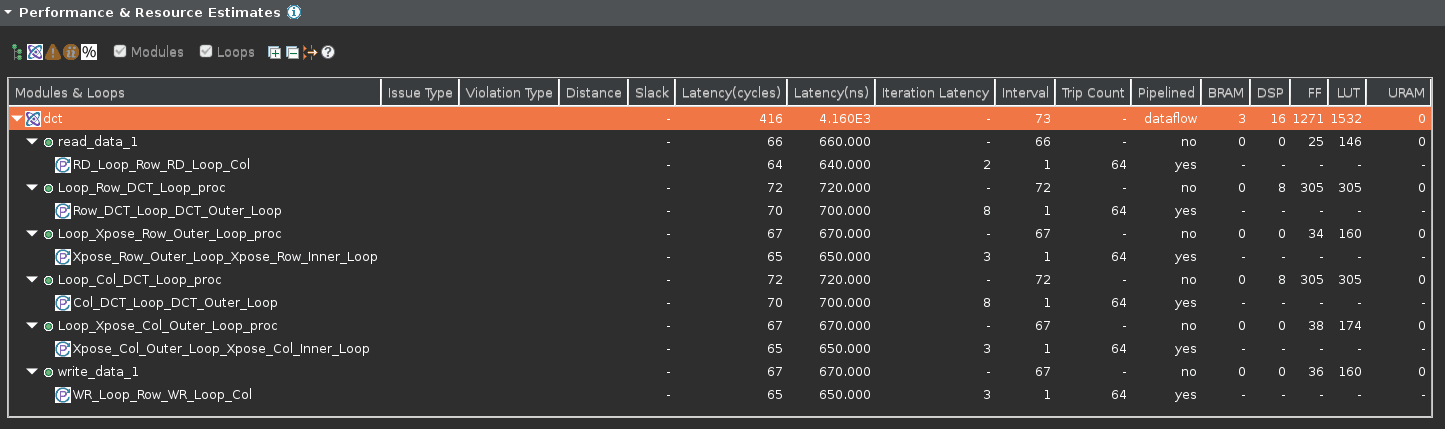
Performance analysis after the INLINE directive
- Close Vitis HLS by selecting File > Exit.
Conclusion
In this lab, you learned various techniques to improve the performance and balance resource utilization. PIPELINE directive when applied to outer loop will automatically cause the inner loop to unroll. When a loop is unrolled, resources utilization increases as operations are done concurrently. Partitioning memory may improve performance but will increase BRAM utilization. When INLINE directive is applied to a function, the lower level hierarchy is automatically dissolved. When DATAFLOW directive is applied, the default memory buffers (of ping-pong type) are automatically inserted between the top-level functions and loops. The console logs can provide insight on what is going on.
Answers
Answers for question 1:
Estimated clock period: 6.508 ns
Worst case latency: 423 clock cycles
Number of DSP48E used: 17
Number of BRAMs used: 16
Number of FFs used: 929
Number of LUTs used: 2012
Copyright© 2022, Advanced Micro Devices, Inc.