Xilinx MC European Engine Benchmark
Xilinx XF_FINTECH Test
This is a benchmark of MC (Monte-Carlo) European Engine using the Xilinx Vitis environment to compare with QuantLib. It supports software and hardware emulation as well as running the hardware accelerator on the AWS F1.
Design
Overview
The European option pricing engine uses Monte Carlo Simulation to estimate the value of European Option. Here, we assume the process of asset pricing applies to Black-Scholes process.
The essence of Monte Carlo Method is the law of large numbers. It uses statistics sampling to approximate the expectation.
It simulates the stochastic process of value of underlying asset. When using Monte Carlo to price the option, the simulation generates a large amount of price paths for underlying asset and then calculates the payoff based on the associated exercise style. These payoff values are averaged and discounted to today. The result is the value to the option today.
Most of the time, the value of underlying asset are affected by multiple factors, and it don’t have a theoretical analytic solution. For this scenario, Monte Carlo Methods are very suitable.
European option is a kind of vanilla option and not path dependent. The option has the right but not the obligation, to be exercised at the maturity time. That is to say, the payoff is only related to the price of the underlying asset at the maturity time.
The payoff is calculated as follows: - payoff of Call Option =
:math:max(S-K,0) - payoff of Put Option = :math:max(K-S,0) Where
:math:K is the strike value and :math:S is the spot price of
underlying asset at maturity time.
Implementation
In Monte Carlo Framework, the path generator is specified with
Black-Scholes. For path pricer, it fetches the logS from the input
stream, calculates the payoff based on above formula and discounts it to
time 0 for option price.
The framework of Monte Carlo Simulations is as follows. The top module Monte Carlo Simulation will call the Monte Carlo Module (MCM) multiple times until it reaches the required samples number or required tolerance.
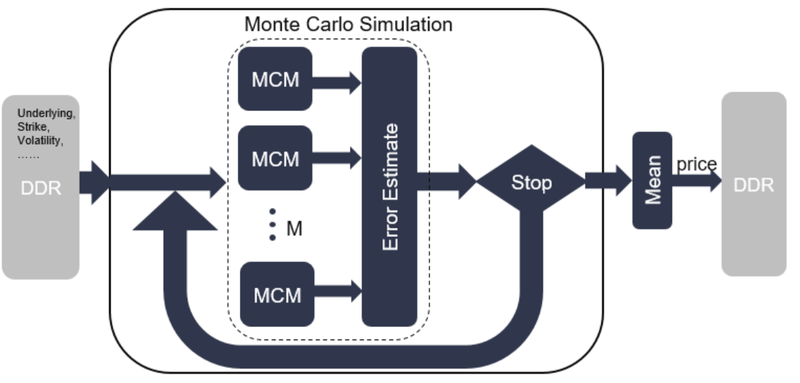
monte Carlo Simulation
Every MCM generates a batch of paths. The number of MCM (M) is a template parameter, the maximum of which is related to the FPGA resource. Each MCM includes an RNG module, a path generator module, a path pricer module, and an accumulator. All of these modules are in dataflow region and connected with hls::stream.
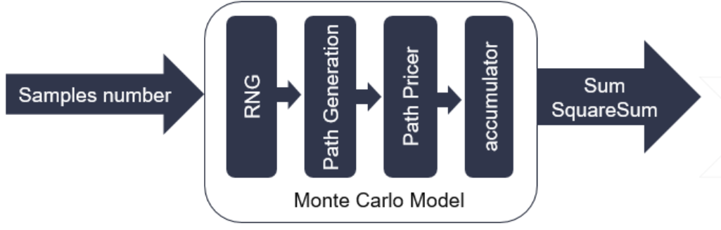
Monte Carlo Model
RNG module generates the normal random numbers. Currently, only generating pseudo-random number is supported. The detailed implementation of RNG inside may refer to the RNG section.
Path Generator uses the random number to calculate the price paths of underlying asset. Currently, Black-Scholes and Heston valuation model are supported.
Path pricer will exercise the option based on the price paths of underlying asset and calculate the payoff, discount the payoff to time zero for option value. Different option has associated implementation for path pricer.
Accumulator sums together the option value and square of option value on all the paths. These sums are prepared for calculation of average and variance. Because the accumulation of floating point data type cannot achieve II = 1, the input is dispatched to 16 sub-accumulator and sum the result of 16 sub-accumulator at last.
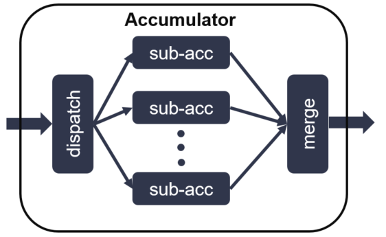
Accumulator
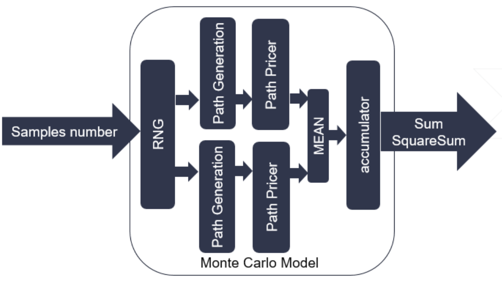
Antithetic paths
Antithetic paths is a kind of variance reduction techniques.
The precision of Monte Carlo Simulation is related with the simulations
times. The error of results is an order of
O(:math:\frac{1}{\sqrt{N}}).
If :math:X applies to :math:\phi(0,1), then the antithetic
variable of is :math:-X. We can call :math:X and :math:-X as
an antithetic pair. In our implementation, when the antithetic template
parameter is set to true. The RNG module will generate two random number
at one clock cycles. Then, two path generators are followed to make sure
it can consume two random number at on clock cycles. At the same time,
the two price paths are averaged at path pricer. The structure with
antithetic is as follows.
The advantage of antithetic paths is not only reducing the number of generated random number from 2N to N, but also reduces the variance of samples paths and improves the accuracy if the correlation of two antithetic variables is negative.
Monte Carlo Model
Prerequisites
Xilinx Vitis 19.2 installed and configured
Xilinx runtime (XRT) installed
Building
The demonstration application and kernel is built using a command line Makefile flow.
Step 1 :
Setup the build environment using the Vitis and XRT scripts:
source <install path>/Vitis/2019.2/settings64.sh
source /opt/xilinx/xrt/setup.sh
Step 2 :
Call the Makefile. For example:
make run DEVICE=xilinx_aws-vu9p-f1_shell-v04261818_201920_1 TARGET=hw
The Makefile supports software emulation, hardware emulation and hardware targets (‘sw_emu’, ‘hw_emu’ and ‘hw’, respectively).
In the case of the software and hardware emulations, the Makefile will build and launch the host code as part of the run. These can be rerun manually using the following pattern:
<host application> <xclbin>
For example example to run a prebuilt software emulation output (assuming the standard build directories):
build_dir.sw_emu.xilinx_aws-vu9p-f1_shell-v04261818_201920_1/test.exe -xclbin build_dir.sw_emu.xilinx_aws-vu9p-f1_shell-v04261818_201920_1/kernel_mc.xclbin
AWS
for AWS F1 platform, it needs to convert xclbin to awsxclbin (https://github.com/aws/aws-fpga and https://github.com/aws/aws-fpga/blob/master/Vitis/README.md), then run:
./bin/test.exe -xclbin xclbin/awsxclbin
Output
for the testbench, process it via the engine and compare to the expected result, displaying the case difference. For example:
----------------------MC(European) Engine-----------------
Found Platform
Platform Name: Xilinx
Selected Device xilinx_aws-vu9p-f1_dynamic_5_0
INFO: Importing kernel_mc_xilinx_aws-vu9p-f1_shell-v04261818_201920_1.awsxclbin
Loading: 'kernel_mc_xilinx_aws-vu9p-f1_shell-v04261818_201920_1.awsxclbin'
loop_nm = 1024
num_rep = 20
cu_number = 3
kernel has been created
FPGA execution time: 0.515286 s
option number: 20480
opt/sec: 39744.9
Expected value: 3.833452
FPGA result:
            Kernel 0 - 3.85041
            Kernel 1 - 3.86199
            Kernel 2 - 3.84573
EXCLUDED PLATFORMS
Platforms containing following strings in their names are not supported for this example :
_u25_
u30
u50
u200
u280
zc
qdma
vck
samsung
_u2_
nodma
DESIGN FILES
Application code is located in the src directory. Accelerator binary files will be compiled to the xclbin directory. The xclbin directory is required by the Makefile and its contents will be filled during compilation. A listing of all the files in this example is shown below
src/kernel_mc.cpp
src/kernel_mceuropeanengine.hpp
src/test.cpp
src/utils.hpp
src/xcl2.cpp
src/xcl2.hpp
src/xcl2.mk
Access these files in the github repo by clicking here.
COMMAND LINE ARGUMENTS
Once the environment has been configured, the application can be executed by
./test.exe -xclbin <kernel_mc XCLBIN>