GQE Kernel Design
Caution
There is NO long-term-support to current version GQE kernels. The kernel APIs are subject to be changed for practicality in the comimg release.
Join Kernel
The GQE join kernel is a compound of multiple post-bitstream programmable primitives, and can execute not only hash-join but also a number of primitives often found as prologue or epilogue of join operations. With its bypass design in data path, it can even perform execution without a join.
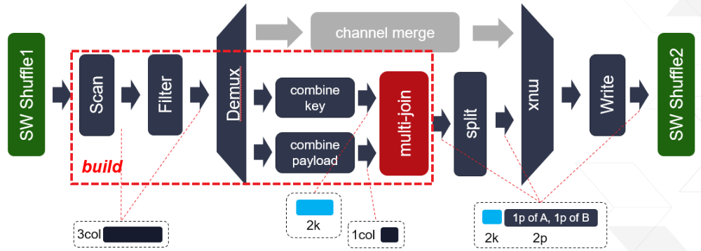
The internal of this kernel is illustrated in the figure above. Internal multi-join supports three reconfigurable modes, namely inner join, anti-join and semi-join. To join efficiently at different data scale, the join process is divided into two phases: build and probe. Build phase takes Table A as input to build the hash table, while Probe phase takes Table B as input and probes the conflicting rows from built hash table. By calling Table B multiple iterations, any sized Table B can be joined. On the other hand, By spliting Table A into multiple slice and running mutli-(build + Nx probe), Table A with any size can be employed as the left table.
This kernel works with three types of input buffers, 1x kernel configuration buffer, 1x meta info buffer and 3x column data buffers. The result buffers are 1x result data meta and 4x output column data.
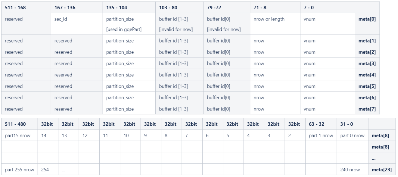
The input / output data columns save all raw column data. The statistic information, e.g., row number, column number, is recorded in meta input / output buffer. The internal structure of meta info is shown in the figure below. The first 4 rows are valid for Join kernel. Each row represents the info of one data column.
Note
- gqePart kernel supports maximum 256 partitions, each partition nrow is 32-bit, starting from meta[8], 256 / 16 = 16 lines are used for partitioning nrow output.
- When the partition num is less than 256, using the first N parts, starting from meta[8][31-0]
Caution
In the current release, all columns are expected to have the same number of elements of same type.
The configuration buffer basically programs the kernel at runtime. It toggles execution step primitives on or off, and defines the filter and/or evaluation expressions. The details are documented in the following figure:
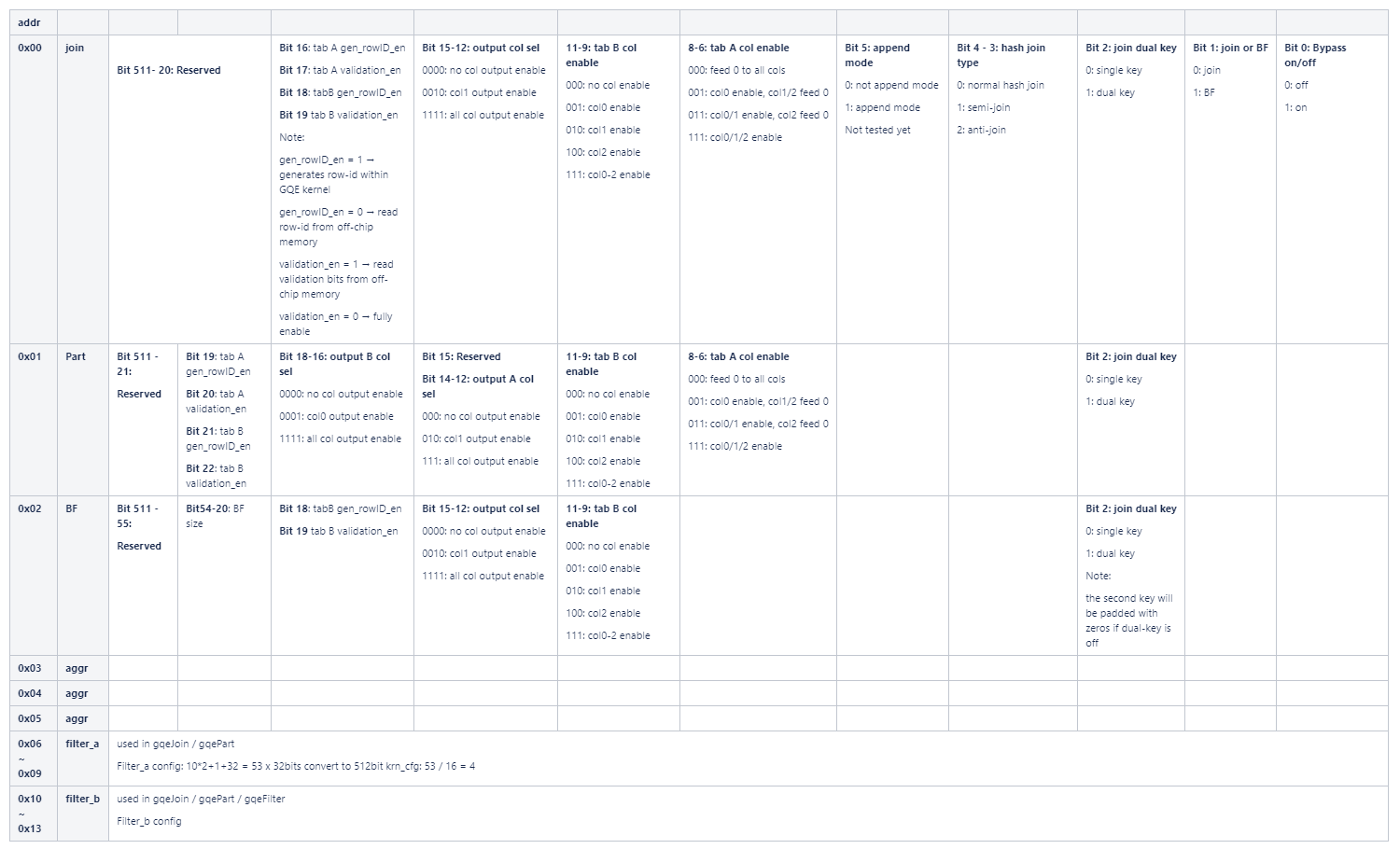
14 lines of 512-bit configure data are used in kernel command. Address 0x00 is join only config, 0x01 for partition kernel, 0x02 for bloomfilter kernel, and 0x03-0x05 is reserved for gqeAggr kernel. Since the filtering module is the same in all kernels, same configuration lines 0x06 - 0x13 are used.
Both input table A and B can support up to 3 columns, which may consist of 1-2 key columns and 1 payload columns. The col enable flags are set in bit 6-11. The output column enable flags are 12-15 bits.
Payload column data, which is normally used as rowID column, can be read from user input or auto-generating in kernel. The rowID generation config is controled by bit16/18. If generating rowID inside the kernel, the validation enable flag also must be configured to determin whether to use the validation buffer.
The columns are indexed starting from 0. -1 is used as a special value to instruct the table scanner to feed zero for that column.
Current kernel join kernel can be configured to join mode or bloomfilter mode, which is controlled by bit 1.
The filter config is aligned to lower bits. Build/probe table’s filter config are located in addr 0x06-0x09 / 0x10-0x13.
The join_on option toggles whether hash-join is enabled or by-passed in the pipeline.
The dual_key option instructs the kernel to use both first and second column as join key in hash-join, and when it is asserted, the third column
becomes the first part of the payload input.
The join sel option indicates the work mode of multi-join, 0 for normal hash join, 1 for semi-join and 2 for anti-join.
Caution
The 3-columns input data are scanned in via 3x 256-bit AXI ports. However, only 1x 512-bit AXI port is employed to output (up to_ 4 cols data. When the resulting data are huge, the write out module performance would decrease the kernel performance.
Note
Directly bypass is supported by configuring the join kernel to probe mode. Then the kernel works as a filtering kernel. All data will go through the “channel merge” path in the kernel structure figure shown on the top.
The hardware resource utilization of join kernel is shown in the table below (work at 180MHz).
| Module | LUT | LUT as memory | Register | BRAM36 | URAM | DSP |
| AXI adapters | 53546 | 23316 | 79997 | 156.5 | 0 | 0 |
| Scan | 8402 | 931 | 10032 | 1 | 0 | 0 |
| Filter | 20496 | 3936 | 12629 | 0 | 0 | 0 |
| crossbar 4-to-8 | 7166 | 729 | 11653 | 0 | 0 | 0 |
| join (BF) | 12375 | 2659 | 15272 | 9.5 | 24 | 12 |
| collect 8-to-1 | 608 | 0 | 2110 | 0 | 0 | 0 |
| Write | 7687 | 8 | 6738 | 30 | 0 | 0 |
| Total | 110280 | 31579 | 138431 | 197 | 24 | 12 |
Bloom-Filter Kernel
The bloom-filter is a space-efficient probabilistic data structure that is used to test whether an element is a member of a set. False positive matches are possible, but false negatives are not - in other words, a query returns either “possibly in set” or “definitely not in set”. (from Wikipedia)
The GQE Bloom-Filter kernel is an HLS kernel implementation that fully utilizes the high bandwidth feature of HBM to accelerate the query (probe-only) ability and expands the capacity as large as possible at the same time.
The GQE Bloom-Filter kernel also shares the same framework as GQE Join. Thus, the input key and payload should be 64-bit width, and 1 or 2 key column(s) plus 1 playoad column is allowed to be applied to the kernel. In addition, the bloom-filter and join functionality selection is controlled by kernel command bit config[0][1], where bloom-filter is enabled by setting the corresponding bit to 1.
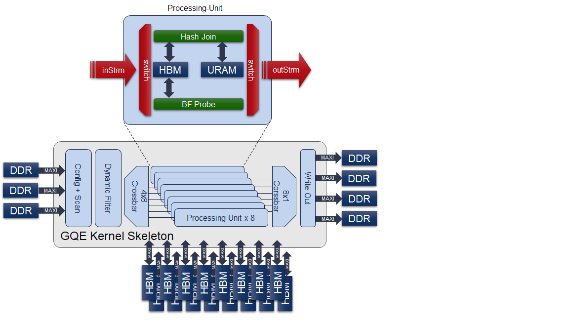
The structure of the gqeJoin (bloom-filter) can be shown as the following figure:
As the main usage of the GQE kernel is already covered in GQE Join kernel design. We’ll only introduce the specifications for input and output columns of GQE for using bloom-filter flow here.
The columns for using the bloom-filter flow can be explained as:
| Input | Column 0 | key 0 |
| Column 1 | key 1 (if dual-key is enabled) | |
| Column 2 | payload | |
| Output | Column 0 | payload |
| Column 1 | unused (no additional payload in bloom-filter flow) | |
| Column 2 | key 0 | |
| Column 3 | key 1 (if dual-key is enabled) |
Software developer who wants to benefit from the hardware acceleration for bloom-filtering, please kindly refer to the Example Usage in L3 documentation.
Aggregate Kernel
The Aggregate kernel is another key kernel of General Query Engine (GQE) which supports both grouping and non-grouping aggregate operations.
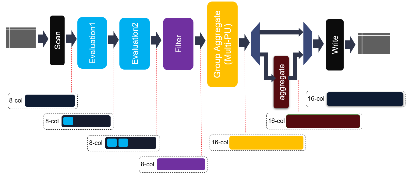
The internal structure of this kernel is shown in the figure above. Same to join kernel, 8-cols data buffer, 1x kernel config buffer and 1x meta info buffer are employecd as the kernel input. Due to the diversity of output data types, e.g., aggregate max, min, raw data, etc., 16x output column buffers are used as the output buffer. As shown in above figure, before entering into hash group aggregate module, each element in each row will be evaluated and filtered. Thus, some new elements can be generated and some rows will be discarded. Moreover, two cascaded evaluation modules are added to support more complex expression.
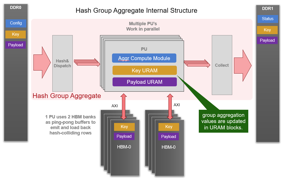
The core module of aggregate kernel is hash group aggregate, which is a multi-PU implementation and given in the following diagram. Each PU requires 2 HBM banks and some URAM memory blocks to buffer distinct keys as well as payloads after aggregate operations. And one internal loop is implemented to consume all input rows with each iteration. Furthermore, all PUs are working in parallel to achieve higher performance.
The data structure of input and output meta and raw data are same as join kernel. The configuration buffer is composed of 128x 32-bit slots. The details of configuration buffers are listed in the table:
| Module | Module Config Width | Position |
| Scan | 64 bit | config[0]~config[1] |
| Eval0 | 289 bit | config[2]~config[11] |
| Eval1 | 289 bit | config[12]~config[21] |
| Filter | 45*32 bit | config[22]~config[66] |
| Shuffle0 | 64 bit | config[67]~config[68] |
| Shuffle1 | 64 bit | config[69]~config[70] |
| Shuffle2 | 64 bit | config[71]~config[72] |
| Shuffle3 | 64 bit | config[73]~config[74] |
| Group Aggr | 4*32 bit | config[75]~config[78] |
| Column Merge | 64 bit | config[79]~config[80] |
| Aggregate | 1 bit | config[81] |
| Write | 16 bit | config[82] |
| Reserved | config[83]~config[127] |
The hardware resource utilization of hash group aggregate is shown in the table below (work as 180MHz).
| Primitive | Quantity | LUT | LUT as memory | LUT as logic | Register | BRAM36 | URAM | DSP |
| Scan | 1 | 12209 | 4758 | 7451 | 18974 | 0 | 0 | 2 |
| Eval | 8 | 2153 | 426 | 1727 | 2042 | 4 | 0 | 21 |
| Filter | 4 | 2168 | 13 | 2155 | 1764 | 0.5 | 0 | 0 |
| Group Aggr | 1 | 162202 | 27819 | 134383 | 210926 | 62 | 256 | 0 |
| Direct Aggr | 1 | 4349 | 0 | 4349 | 6611 | 0 | 0 | 0 |
| Write | 1 | 30938 | 9490 | 21448 | 43579 | 0 | 0 | 0 |
| AXI DDR | 1 | 4586 | 1313 | 3273 | 78855 | 18 | 0 | 0 |
| AXI HBM | 1 | 20528 | 4456 | 16072 | 45416 | 124 | 0 | 0 |
| Total | 298470 | 60402 | 238068 | 399737 | 255 | 256 | 2 |
Partition Kernel
The GQE partition kernel can partition one table’s rows into corresponding clusters according to hash of selected key columns. This kernel is designed to scale the problem size that can be handled by the GQE Join or Aggregate kernel. To reduce the size of intermediate data, it is equipped with dynamic filter like other kernels.
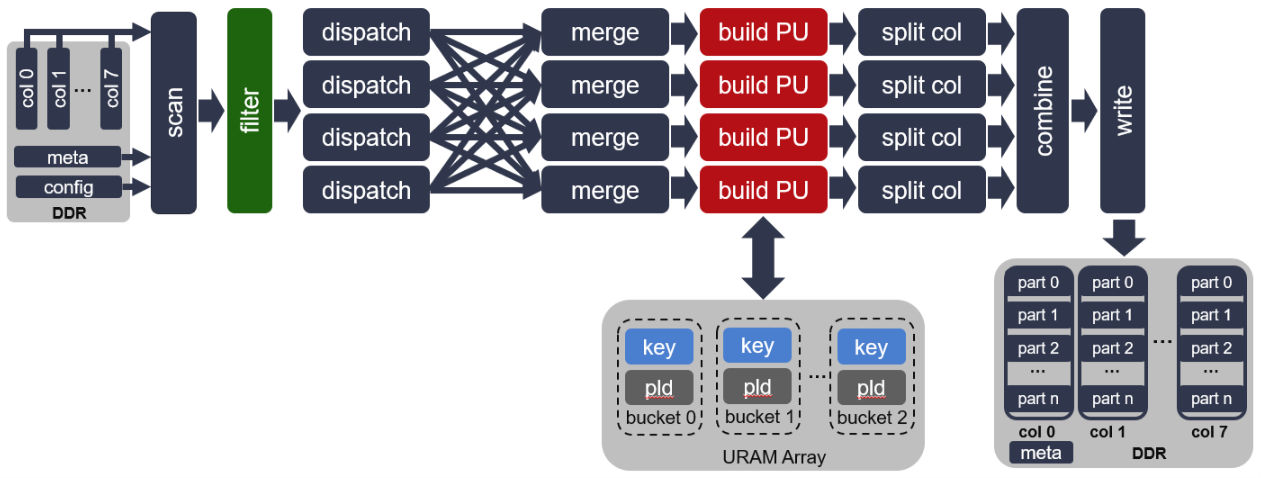
The internal of this kernel is illustrated in the figure above. It scans kernel config buffer, metainfo buffer and 8x cols input raw data in and passes to a filter. The filter condition is configured in kernel config buffer. After filtering, each row data will be dispatched into one of 4 PUs to calculate hash value of the primary key. Based on the hash value, the key and payload data are saved to the accroding bucket / partition. Once one bucket is full, the full bucket will trigger one time burst write which writes data from bucket to resulting buffer.
In the kernel structure, URAM array that connected to “build PU” is drawn. Here maximum 256 buckets are created in URAM array, each bucket saves one time burst write to resulting buffer. The output of partition kernel is 8x cols output data and 1x meta info buffer.
To simplify the design, GQE partition kernel can reuse the scan and filter configuration with GQE join kernel. Also, as mentioned above, the data structure of input and output tables is the same as join kernel.
The hardware resource utilization of single hash partition is shown in the table below (work as 200MHz).
| Primitive | LUT | LUT as memory | LUT as logic | Register | BRAM36 | URAM | DSP |
| Scan | 17109 | 5400 | 11709 | 20538 | 0 | 0 | 0 |
| Filter | 12853 | 3300 | 9553 | 8106 | 0 | 0 | 0 |
| Hash partition | 64336 | 5424 | 59912 | 50573 | 122 | 208 | 20 |
| Write | 22385 | 5082 | 4816 | 29608 | 9 | 0 | 3 |
| AXI DDR | 37917 | 3461 | 34456 | 42380 | 51 | 0 | 6 |
| Total | 134818 | 26553 | 108220 | 116884 | 240 | 256 | 29 |
Attention
For gqeJoin and gqeAggr kernel, only first 8 rows are valid. However, all 24 rows are valid in gqePart kernel. The row number of each output partition is given in the output meta, from row 8 to 23. Due to the supported maximum partition number is 256, each row number takes 32 bit in meta buffer, 256/(512/32) = 16 lines are employed to save these row number info. Besides, The partition size should be provided for gqePart input meta.