Finite Difference Methods
Overview
Finite Difference Methods are a family of numerical techniques to solve partial differential equations (PDEs). They do this by discretizing the continuous equation in the spatial dimensions (forming a multidimensional grid), and then iteratively evolving the system over a series of N discrete time steps. The result is a discrete solution for each individual grid point.
In the provided solver, the PDE is the Heston Pricing Model [HESTON1993]. Using the naming conventions of Hout & Foulon [HOUT2010], the PDE is given as:
Where:
\(u\) - the price of the European option;
\(s\) - the underlying price of the asset;
\(v\) - the volatility of the underlying price;
\(\sigma\) - the volatility of the volatility;
\(\rho\) - the correlation of Weiner processes;
\(\kappa\) - the mean-reversion rate;
\(\eta\) - the long term mean.
The Heston PDE then describes the evolution of an option price over time (\(t\)) and a solution of this PDE results in the specific option price for an \((s,v)\) pair for a given maturity date \(T\). The finite difference solver maps the \((s,v)\) pair onto a 2D discrete grid, and solves for option price \(u(s,v)\) after \(N\) time-steps.
Implementation
The included implementation uses a Douglas Alternating Direction Implicit (ADI) method to solve the PDE [DOUGLAS1962]. Implicit methods are needed to provide a stable and useful solution, and the Douglas solver is the most direct of these methods.
Assumptions/Limitations
The following limitations apply to this implementation:
- The dividend yield term (\(r_f\) above) is fixed to zero;
- Boundary conditions are fixed in time.
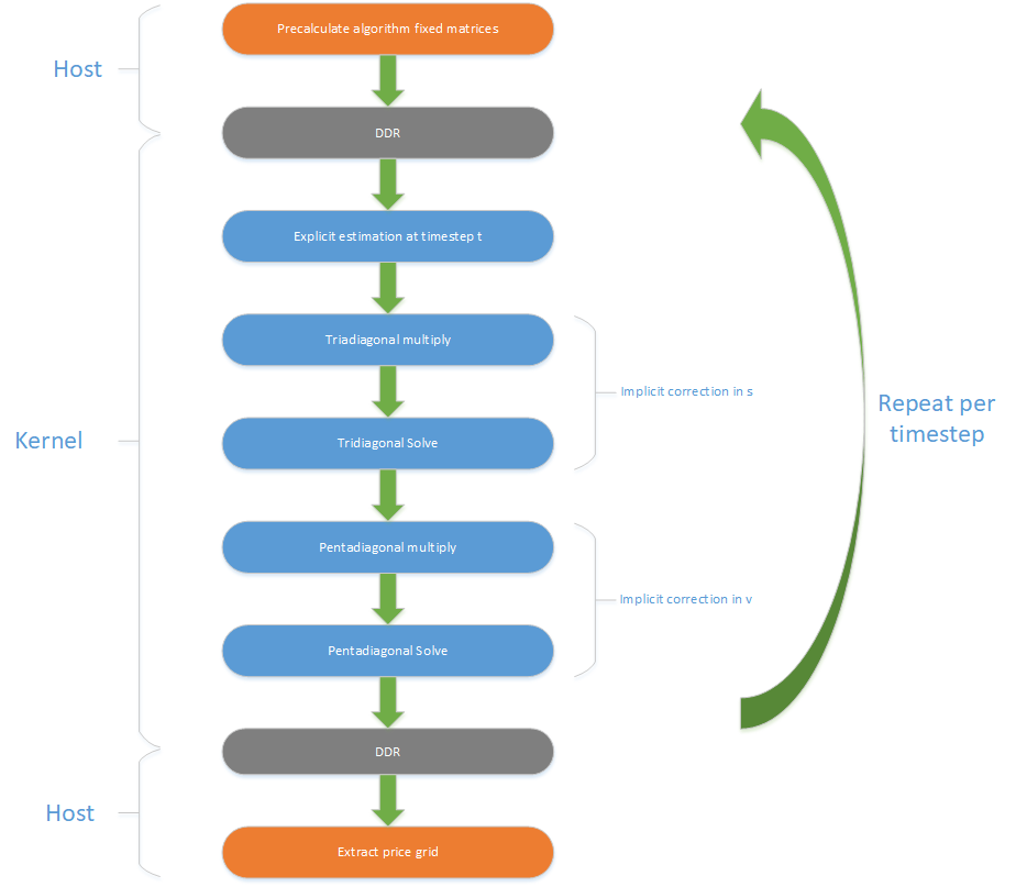
Dataflow Description
Precalculate algorithm fixed matrices
A function in the host software generates the finite-difference grid (possibly non-uniform) and the \(\alpha\), \(\beta\), \(\gamma\) and \(\delta\) coefficients based on the grid. These are converted into a set of \(\mathbf{A}\) matrices (in sparse form) and \(\mathbf{b}\) boundary vectors, plus modified forms of the \(\mathbf{A}\) matrices for the tridiagonal and pentadiagonal solvers (the \(\mathbf{X}\) matrices). The initial condition of the grid is also calculated on the host, and all of these cofficients are moved into the DDR memory on the Alveo card.
The following three steps are performed in hardware on the Alveo card for each timestep of the simulation.
Explicit estimation at timestep t
A direct estimate of the PDE at the next timestep is made using the current values for the grid coefficients.
Implicit correction in s
The estimate is corrected using the new values in the PDE in the s direction. This takes the form of a multiplication by a tridiagonal matrix and then a subsequent tridiagonal solve.
Implicit correction in v
The estimate is then corrected using the new values in the PDE in the v direction. This takes the form of a multiplication by a pentadiagonal matrix and then a subsequent pentadiagonal solve.
Extract price grid
On completion of the simulation of all timesteps on the Alveo card, the host moves the final grid values back from the DDR memory and then extracts the final pricing information from those grid values.
References
| [HESTON1993] | Heston, “A closed-form solution for options with stochastic volatility with applications to bond and currency options”, Rev. Finan. Stud. Vol. 6 (1993) |
| [HOUT2010] | Hout and Foulon, “ADI Finite Difference Schemes for Option Pricing in the Heston Model with correlation”, International Journal of Numerical Analysis and Modeling, Vol 7, Number 2 (2010). |
| [DOUGLAS1962] | Douglas Jr., J, “Alternating direction methods for three space variables”, Numerische Mathematik, 4(1), pp41-63 (1962). |