Internal Design of Black Scholes Local Volatility Solver

Overview

Black-Scholes models the dynamics of a financial market containing derivative investment instruments. It is described by the following Partial Differential Equation (PDE)

\[\frac{\partial U}{\partial t} + \frac{1}{2} \sigma^2 S^2 \frac{\partial^2 U}{\partial S^2} + rS \frac{\partial U}{\partial S} - rU = 0\]

The model assumes a constant volatility and risk-free rate. The model can be generalized to remove this restriction.This form of the equation can be use to price options using a local volatility description.

\[\frac{\partial U}{\partial t} + \frac{1}{2} \sigma^2(S,t) S^2 \frac{\partial^2 U}{\partial S^2} + r(t)S \frac{\partial U}{\partial S} - r(t)U = 0\]

Mathematical Background

The engine makes use of a finite difference approach to solve the generalized Black Scholes model. The first step is to reformulate the equation to evolve backwards in time such that the known final state (the payoff) can be used as the initial condition. To do this set

\[\tau = T-t\]

such that

\[\frac{\partial U}{\partial \tau} = - \frac{\partial U}{\partial t}\]

Which leads to

\[\frac{\partial U}{\partial \tau}=\frac{1}{2} \sigma^2(S,\tau) S^2 \frac{\partial^2 U}{\partial S^2} + r(\tau)S \frac{\partial U}{\partial S} - r(\tau)U\]

In order to facilitate the use of a standardize finite difference solver, the Black Scholes equation is reformulated into a standard form (similar to the Heat Equation) by making the substitution

\[x = log(S)\]

Following the standard variable substitution technique

\[\frac{\partial U}{\partial S} = \frac{\partial U}{\partial x} \frac{\partial x}{\partial S} = \frac{1}{S}\frac{\partial U}{\partial x}\]

and

\[\frac{\partial^2 U}{\partial S^2} = \frac{1}{S}\frac{\partial}{\partial x}\Bigg(\frac{1}{S}\frac{\partial U}{\partial x}\Bigg)\]

which can be evaulated using the product rule and knowing that

\[\frac{1}{S} = e^{-x}\]

To give

\[\frac{\partial^2 U}{\partial S^2} = \frac{1}{S^2}\frac{\partial^2 U}{\partial x^2} - \frac{1}{S^2}\frac{\partial U}{\partial x}\]

Plugging this into the backwards evolving equation (the S, t dependence is herein implied)

\[\frac{\partial U}{\partial \tau}=\frac{1}{2} \sigma^2 S^2 \Bigg (\frac{1}{S^2}\frac{\partial^2 U}{\partial x^2} - \frac{1}{S^2}\frac{\partial U}{\partial x} \Bigg) \frac{\partial^2 U}{\partial S^2} + rS \frac{\partial U}{\partial S} - rU\]

which simplifies to

\[\frac{\partial U}{\partial \tau}=\frac{1}{2} \sigma^2 \frac{\partial^2 U}{\partial x^2} + (r-\frac{1}{2} \sigma^2)\frac{\partial U}{\partial x} - rU\]

This is clearly of the form

\[\frac{\partial U}{\partial \tau}=A \frac{\partial^2 U}{\partial x^2} + B\frac{\partial U}{\partial x} +CU\]

with

\[A = \frac{1}{2} \sigma^2 , B= (r-\frac{1}{2} \sigma^2) , C=-r\]

This transformed equation is then approximated by standard central difference equations but allowing for non-uniform spatial discretization.

\[\frac{\partial U}{\partial x}=\frac{U_{i+1} - U_{i-1}}{h_i + h_{i+1}}\]

\[\frac{\partial^2 U}{\partial x^2}=\frac{1}{h_i + h_{i+1}}\Bigg(\frac{U_{i+1} - U_{i}}{h_{i+1}} - \frac{U_{i} - U_{i-1}}{h_{i}}\Bigg)\]

where

\[h_i = x_i - x_{i-1}\]

The tempororal discretization is simply

\[\frac{\partial U}{\partial \tau}=\frac{U^{j+1} - U^{j}}{\tau}\]

where the time-step is a linear grid from 0 to T (maturity date) in M steps.

Design Details

The general structure of the solver is shown below:

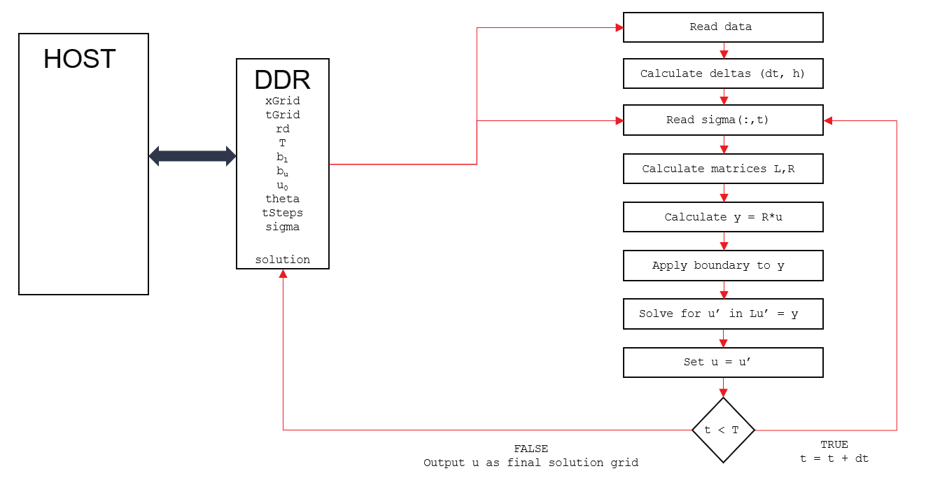
The hardware design is parameterized with sizes N, M via the Makefile (see README.md in the FDBlackScholesLocalVolatility test directory). N is the number of grid points in the spatial (x) direction. This number in turn governs all of the internal vector and matrix sizing. M is the maximum number of time steps which can be supported by this particular parameterized build, but it is possible to pass in a smaller time-step value (tSteps) at runtime (with corresponding reductions in the data vectors). The host code provides the discrete grid points x[N], t[M] (remember that x=log(S) for this solver). Additionally, the host provides the maturity date T (in years), risk-free rate r[M], sigma[N*M] evaluated at each grid point in the x,t mesh, initial condition u[N], and the upper and lower boundary conditions to match the initial condition.

The engine will then calculate the dt, h deltas (a one-time step). Then, at each time step dt, the left and right hand matrices for the linear system Lu’ = Ru are calculated, where u is the current solution grid, u’ is the next time-step solution. Due to the use of central-differencing and the Dirichlet boundary conditions, these will be tridiagonal matrices. The right-hand side Ru is calculated (a simple tridiagonal array by vector multiplication) and the suitably discounted boundary conditions are applied. Finally the linear system is solved to get u’ which becomes u in the next iteration. Because of the tridiagonal matrices, the linear system is solved by making use of the efficient Parallel-Cyclic-Reduction (PCR) engine found in the L1 library.

Note that the engine supports selection of the solver method implemented via the Theta parameter which should be set to 0 for explit, 1 for fully-implicit, or 0.5 for Crank-Nicholson. Other values in the range 0 to 1 can be freely selected but are not commonly used.

Test Methodology

The Finite Difference solver is verified by using a separate Python implementation which is compared to results from the scikit-fdiff PDE solver across a range of different test cases. This allows for fast verification of the solver design. Once this was complete, the HLS design is executed against the same test cases and the output is compared to a reference solution generated by the Python model. Ideally, these would match precisely; in practise small differences of around 10^-4 are seen due to the use of floating point data types and hardware optimised operator ordering in the HLS version.

Three test cases are providing for confirming the engine is working correctly. These are to be used with the default N=128 M=256 build.

case 0 - Vanilla European

This is a special case where the volatility is constant in both time and price dimensions, and the risk-free rate is constant. This is the standard Black-Scholes model and in this case, there is a closed form solution which allows the final result to be independently confirmed.

case 1 - Volatility Smile

This case has a time and spatially varying volatility surface

case 2 - Severe Spatial Surface

This case has a volatility surface where the volatility follows a sine wave in the spatial direction. This is unrealistic but designed to check the stability of the solver.