Internal Design of Heath-Jarrow-Morton Framework
Overview
The Heath-Jarrow-Morton (HJM) framework is a general framework to model the evolution of instantaneous forward rate curves. The paths generated by the HJM framework are non-Markovian and its implementation is solved by Monte-Carlo simulation. We provide a multi-factor Monte-Carlo implementation of the HJM framework, where the volatilities can be calculated by performing a Principal Component Analysis of historical interest rate curves.
Note that calculations based on the HJM Framework are by nature a long-running process and hardware emulation of an HJM-based kernel may take several days to complete.
Design Structure
For a given tenor structure \(T_0,T_1,...,T_n\) evenly spaced with \(\tau = T_{i+1} - T_{i}, \forall i=1,...,n\) we need to calculate the calibrated drift and volatilities for the simulation of future forward rate curves. In order to achieve that, the full implementation of the HJM framework consists in 2 main parts:
PCA HJM Kernel
This sub-kernel deals with the calibration and calculation of the volatility vectors and drift component for the Monte-Carlo simulation. Takes as an input a matrix representing historical data, arranged in a set of vectors \(k\) tenors wide with historical observations going from \(m\) days in the past up to today’s forward curve. For better numerical results, the framework will reduce the historical data into 3 principal components, whose weighted matrix will represent the discrete volatilities for the model. We then approximate each discretised volatility vector with a polynomial. For best results, we have chosen to approximate the first volatility vector with a constant and the remaining two with cubic polynomials.
The outputs are calculated by the following process:
- Calculate the row difference of the historical data matrix \(M\):
- Calculate the loadings matrix of the Principal Component Analysis of the matrix’s delta up to 3 factors. This will represent the 3 discrete volatility vectors, \(k\) elements wide:
- Apply a polynomial fitting to each volatility vector. We will use a constant approximation (D=0) for the first vector and cubic approximation (D=3) for the second and third vector. A polynomial fitting can be calculated by solving by the least-squares approximation the following system of equations:
where \(Y = L_i\) and \(A\) is the vandermonde matrix with \(j = D + 1\) columns and \(x = 0,1,...,n\)
- Applying polynomial fitting to each loadings matrix’s columns we get the polyfitted vectors \(p_1, p_2, p_3\), each vector is \(D_i\) elements wide and represent the coefficients of the polynomial
- From there we get the 3 volatility vectors by evaluating each polynomial at \(x = 0,1,...,n\) tenors.
- For the calculation of the risk neutral drift we take the polyfitted coefficient vectors and calculate the drift vector by evaluating the following function at \(t = 0,1,...,n\):
- Lastly, the MonteCarlo engine requires the present interest rate curve in order to serve as the starting point of the path simulation. This is just the last row from the historical data multiplied by \(dt = 0.01\)
MC HJM Kernel
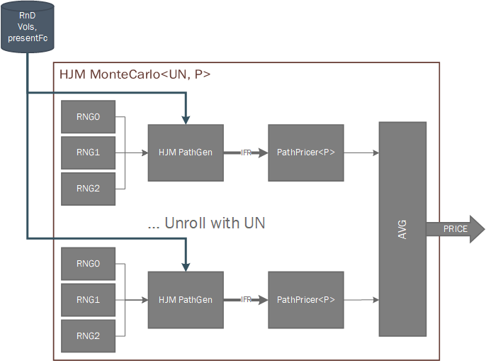
This sub-kernel deals with the different path generations and path pricings. It takes as an input the 3 volatility vectors, the risk neutral drift vector and the present forward curve and generates \(N\) paths, \(k\) tenors wide and \(simYears/dt\) deep consisting on the instantaneous forward rate curves associated at each time-step into the future. Then they are fed into the provided pricer algorithm, which will calculate and output the price per path and the average of all prices is returned to the user. The HJM framework implementation allows to easily set the parallelism level via the UN parameter.
The dynamics of the path generation for the HJM framework follows the equation:
Below there is an Architectural diagram of the HJM MonteCarlo framework as it’s implemented.
Pricer Algorithms
Currently, we support pricing of a ZeroCouponBond with the HJM framework. There are 2 ways of calculating the price of a ZCB at maturity \(t\), via the short rate and the forward curve. Importantly, the forward rate method is an analytical formula depending only on the present forward curve and the time to maturity, so we can use it to calibrate and validate the results from the MonteCarlo HJM framework in order to get confidence for pricing other path-dependent options.
The forward rate ZCB price can be calculated with:
This will give our reference price, which can be compared with the average of \(N\) prices calculated with the short rate of each path via:
After enough iterations, the average values from all the short rate calculations should converge to the value obtained with the forward curve method.