Internal Design of Finite-Difference Hull-White Bermudan Swaption Pricing Engine
Overview
Using the Finite-difference methods (FDM) to estimate the value of Bermudan Swaption. Here, we assume that the floating rate at each time point conforms to Hull-White model.
In Bermudan swaption, the owner is allowed to enter the swap on several pre-specified dates, usually coupon dates of the underlying swap. Notice that we evaluate the value of the swaption as a payer who pay the fixed leg and receive the floating leg of the interest rates.
Implementation
The pricing process of Finite-Difference Hull-White Bermudan Swaption engine is shown in the figure below:
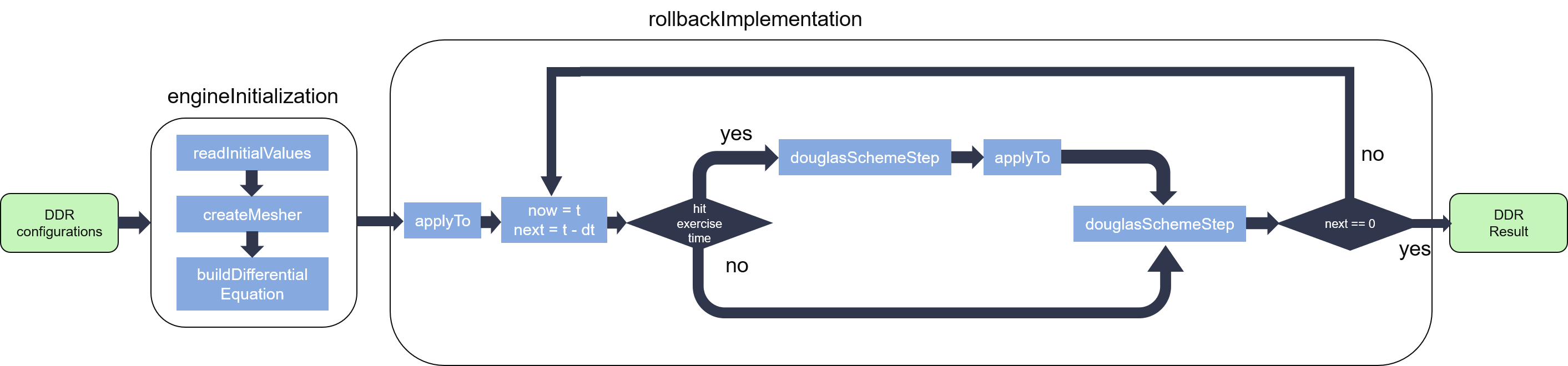
As we can see from the figure, the engine has two main modules: engineInitialization and rollbackImplementation. The former one is responsible for engine initialization, including read specific time points of the swaption from DDR, set initial values, create the mesher using Ornstein-Uhlenbeck process, and build up the second-order differential operator.
After Initialization, the pricing engine evolves back step by step from the last exercise date (maturity) to settlement date (typically \(t=0\)) using FDM, with the \(StepDistance=\frac{maturity - 0}{tGrid}\). Notice that when hitting an exercise time, the engine automatically evolves back from \(now\) to the current exercise time. Meanwhile, the asset price which is stored in \(array\_\) of the engine should be the maximum between its continuation (result evolved by douglasSchemeStep) and the intrinsic value (result calculated with current interest rates at the current exercise time by applyTo), then continue evolving back from current exercise time to the \(next\) time point.
Since engineInitialization process will be executed for only once, while applyTo process will run \(\_ETSize\) times in a single pricing process, additionally, both of them have a latency which is much shorter than douglasSchemeStep process, so they’re optimized for minimum resource utilizations with a reasonable overall latency. But as with douglasSchemeStep process, we try our best to decrease its latency to reduce the whole latency in the pricing process.
Mesher
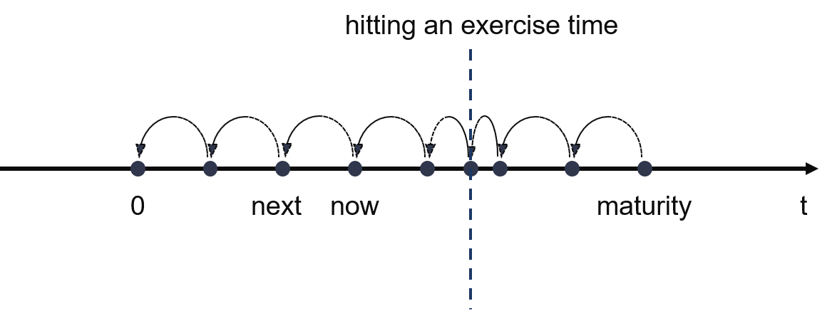
In order to describe the desired range for the underlying value, we utilize the mesher which is stored in \(locations\_\) of the engine to store the discretization of one dimension of the problem domain. In our implementation, we employ Ornstein-Uhlenbeck process to generate the mesher, a sketch of the mesher is shown as the following figure:

Differential operator
In finite-difference methods, a differential operator \(D\) is used to transform a function \(f(x)\) into one of its derivatives, for instance \({f}'(x)\) or \({f}''(x)\). As differentiation is linear, so it can be written as a matrix while using linear algebra methods to solve it. As you know, FDM doesn’t give the exact discretization of the derivative but an approximation, like \({f}'_{i}={f}'(x_{i})+\epsilon _{i}\), notice that the error will decreasing along with the decreasing of the spacing of the grid, say, the tighter the grids (including \(t\) axis and \(x\) axis), the better approximation quality, but the worse simulation duration.
As you may refer to Tylor’s polynomial, we just provide differential operators including the first and the second derivative to obtain a manageable approximation error, they can be defined as:
As we can see from the equations that the value of the derivative at any given index \(i\) only determined by the adjacent three values of the function with the middle of the same index, thus the differential operator can be written as a tridiagonal matrix, like:
To save storage resources and avoid redundant computations, we store the upper, main, and lower diagonals of the matrix in the \(dzMap\_\) of the pricing engine and compute it by Thomson algorithm while evolving back, instead of using a traditional matrix with a large number of zeros and many meaningless additions and multiplications in the pricing process.
Evolution scheme
A partial differential equation (PDE) can be written as:
As mentioned above, a differential operator is used to discretize the derivatives on the right-hand side, while the evolution scheme discretizes the time derivative on the left-hand side.
As you know, finite-difference methods in finance start from a known state \(f(T)\), where \(T\) stand for the maturity of the swaption, and evolve backwards to settlement date \(f(0)\). At each time step, we need to evaluate \(f(t)\) based on \(f(t+\Delta t)\).
The Explicit Euler (EE) scheme can be written as below:
Which can be simplified as:
That only simple matrix multiplication is needed to approximate the equation which is mentioned at the first of this subsection makes the EE scheme becomes the simplest one in FDM.
The Implicit Euler (IE) scheme can be written this way:
Simplified as:
Which makes it a more complex scheme to approximate the PDE.
In our implementation, we adopt a generic template to support different schemes, which can be written as:
The formula transforms to EE scheme if we set \(\theta =0\), and it transforms to IE scheme if we let \(\theta =1\) instead. Any value from 0 to 1 can be used, for example, we give a \(\theta =\frac{1}{2}\) to utilize the Crank-Nicolson scheme.
Profiling
The hardware resource utilizations and timing performance for a single Finite-Difference Hull-White Bermudan Swaption prcing engine with \(\_xGridMax=101\) are listed in Table 9 below:
| BRAM | DSP | FF | LUT | CLB | SRL | clock period(ns) |
| 10 | 487 | 167609 | 103349 | 21520 | 10834 | 3.245 |