Internal Design of Finite-Difference G2 Bermudan Swaption Pricing Engine
Overview
The pricing engine is based on Finite-difference methods (FDM) to estimate the value of Bermudan Swaption. Here, we used the two-additive-factor gaussian (G2) model instead of single-factor Hull-White model. The concept of finite-difference methods is introduced in the article Internal Design of Finite-difference Hull-White Bermudan Swaption Pricing Engine.
For a swaption, the owner is allowed to enter the swap on several pre-specified dates as well as coupon dates of the underlying swap. Notice that we evaluate the value of the swaption as a payer who pay the fixed leg and receive the floating leg of the interest rates.
Implementation
The pricing process of Finite-Difference G2 Bermudan Swaption engine is shown in the figure below:
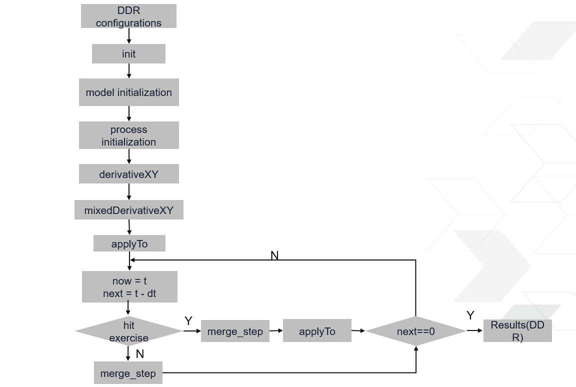
As we can see from the figure, the engine has three main modules: Initialization, calculate and NPV. The former one is responsible for engine initialization: reading specific time points of the swaption from BRAM and setting initial values. The second part is the main process that contains model initialization, meshers initialization using Ornstein-Uhlenbeck process, and builds up the derivative on x and y dimension.
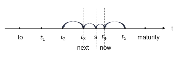
The main logic of the engine is coded in the rollback method. We go backwards from a later time(maturity) to an earlier time in a given number of steps. This gives us a length \(dt\) for each step, which is set as the time step for the evolver. Then we start going back step by step, each time going from the current time t to the next time, \(t-dt\). We have just made the step from \(t_{4}\) to \(t_{3}\) as described in the following paragraph, and it will set the control variable hit to true. It will also decrease the step size of the evolver \(t_{4}-s\). It will lead to the stopping time point, immediately after performing the step. Another similar change of step would happen if there were more than one stopping times in a single step; the code would then step from one to the other. Finally, the code will enter the hitted branch. It performs the remaining step \(s-t_{3}\) and then resets the step of the evolver to the default value.So the process is ready for the next regular step to \(t_{2}\). Notice the last time is \(stopping\_time[1]\) instead of \(stopping\_time[0]\).
Mesher
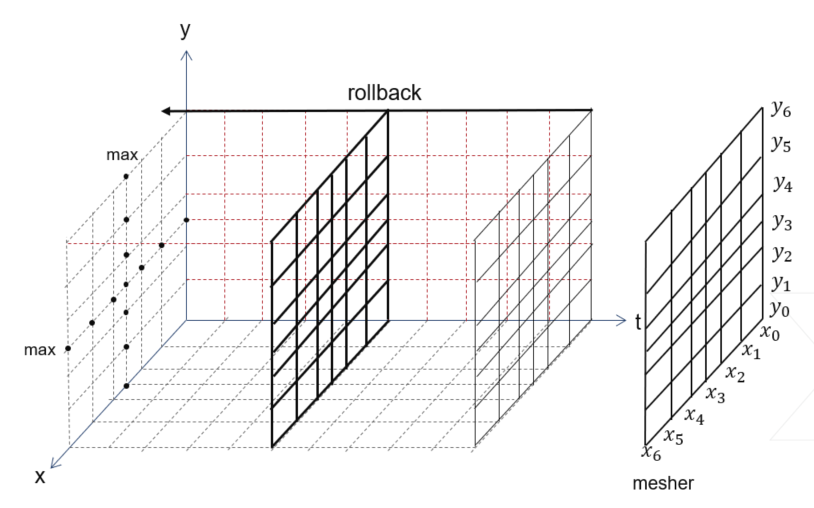
The important component to be build a two-dimensional mesher, which builds the full mesh by composing a 1-D mesh at every dimension of the problem. In the implementation of 2-D mesher, we employ Ornstein-Uhlenbeck process twice with different g2 model arguments. The mesher have two arrays for locations that contain two set of points \(x_{0},x_{1},..,x_{n-1}\) and \(y_{0},y_{1},...,y_{n-1}\) discretizing the domain for x any y. For convenience, it also pre-computes two groups of array dplus and dminus whose i-th elements contain \((x_{i+1}-x_{i})\) and \((x_{i}-x_{i-1})\) respectively. Mesher is shown in the following figure:
As you see, the points in the mesher that we need change the price of the asset. The applyTo method, which modifies the array of asset values in place, must also check that the condition applies at the given time. It would compare the option values to the intrinsic values, and choose the maximum value.
Differential operator
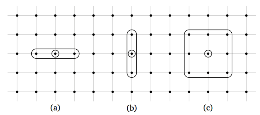
The finite-difference framework defines generic operators for the first and second derivative along a given direction, and we declare the structure named TripleBandLinearOp which contains the lower, diag and upper arrays with the correct values (for instance, the coefficients of \(f(x_{i-1})\), \(f(x_{i})\) and \(f(x_{i+1})\) in the equation for \(\frac{\partial f}{\partial x}(x_{i})\)) based on the 2-D mesher. Here, we also define a structure named NinePointLinearOp which contains the nine neighbors, managing the stencils arguments used in the cross-defivative \(\frac{\partial^{2} f}{\partial x_{i} \partial y_{j}}\) along two directions. The TripleBandLinearOp and NinePointLinearOp are shown in the fugure below. Notice a represents x direction, b represents y direction and c represents nine neighbors.
You may find the details about differential operator and evolution scheme introduced in Internal Design of Finite-difference Hull-White Bermudan Swaption Pricing Engine.
Profiling
The hardware resource utilizations and timing performance for a single finite-difference g2 bermudan swaption prcing engine with \(\_xGrid*\_yGrid*steps=50*50*100\) are listed in Table 10 below:
| BRAM | DSP | FF | LUT | CLB | SRL | clock period(ns) |
| 108 | 535 | 160881 | 158990 | 32294 | 4098 | 3.321 |