Internal Design of American Option Pricing Engine
Overview
The American option can be exercised at any time up until its maturity date. This early exercise feature of American Option gives the investors more freedom to exercise, compared to the European options.
Theory
Because the American option can be exercised anytime prior to the stock’s expire date, exercise price at each time step is required in the process of valuing the optimal exercise. More precisely, the pricing process is as follows:
- Generate independent stock paths
- Start at maturity \(T\) and calculate the exercise price.
- Calculate the exercise price for previous time steps \(T-1\), compare it with the last exercise price, select the larger one.
- Keep rolling back to previous time steps until \(t\) is \(0\) and obtain the max exercise price \(V_t\) as the optimal exercise price.
In the process above, for each time step \(t\), conditional expectation \(E_t[Y_t|S_t]\) of the payoff is computed according to Least-Squares Monte Carlo (LSMC) approach, proposed by Longstaff and Schwartz. Mathematically, these conditional expectations can be expressed as:
where \(t\) is the time prior to maturity, \(B_i(S_t)\) is the basis function of the values of actual stock prices \(S_t\) at time \(t\). The constant coefficients of basis functions are written as \(a_i\) , and acts as weights to the basis functions. The discounted subsequent realized cash flows from continuation called \(Y_t\).
Here we employed polynomial function with weights as the basis functions, so the conditional expectations can be re-written as:
where 3 functions: 1, \(S_t\) and \(S_t^2\) are employed. The constant coefficients \(a\), \(b\) and \(c\) are the weights.
By adding immediate exercise value \(E_t(S_t)\) to the Equation above, and exchanging the side of elements, the equation is changed to
\(a\), \(b\), \(c\), \(d\) are constant coefficients. These coefficients need to be known while calculating the optimal exercise price in mcSimulation model. More details of American-style optimal algorithm used in our library refer to “da Silva, J. N., & Fernández, L. A Monte Carlo Approach to Price American-Bermudan-Style Derivatives.”
Note
Theoretically, the basis functions \(B_i(S_t)\) can be any complex functions and the number of basis function may be any number. The American Option implemented in our library employs three polynomial functions, namely, 1, \(S_t\) and \(S_t^2\), which proved by Longstaff and Schwartz that works well, and is a typical setup in real implementations.
Implementation
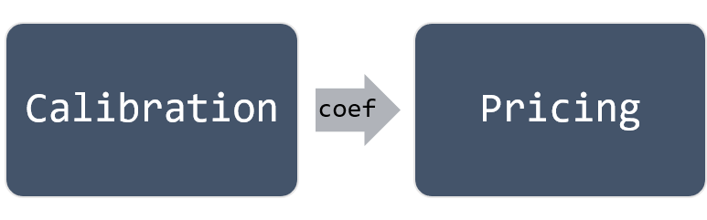
In the Theory Section, the pricing process is described. However, this process can only be executed in the condition of Equation (2) is given. This means that the coefficients in Equation (2) must be calculated first. This calculation process is called Calibration and executes prior to the Pricing process. Therefore, in the implementation, the American Monte Carlo Engine contains two processes: Calibration and Pricing, as illustrated in Figure 10.
- th: 50%
align: center
Hint
Why two processes are required in MCAmericanEngine and only one process, pricing, is enough for European Option Monte Carlo engine?
Calibration Process
Calibration process aims to calculate the coefficients that will be used in the pricing process.
The detailed calculation process is as follows:
- Generate uniform random numbers with Mersenne Twister UNiform MT19937 Random Number Generator (RNG) followed by Inverse Cumulative Normal (ICN) uniform random numbers. Thereafter, generate independent stock paths with the uniform random numbers and Black-Sholes path generator. The default paths (samples) number used in the calibration process is 4096. Thus, 4096 random numbers are generated for each time step \(t\).
- Refer to Equation (2), \(a\), \(b\), \(c\), \(d\) are the unknown coefficients that should be calculated. We denote these coefficients as \(x\), so
The expressions derived from path data \(S_t\), \(S_t^2\) and \(E_t\) can be obtained for each time step \(t\). Here we denote them as \(A\).
Equation (2) can be re-written as:
where \(y\) is the conditional expectation \(E_t(Y_t|S_t)\) in Equation (2). To simplify the expression in deduction, it is denoted as \(y\) in this section. By backward process, this conditional expectation \(y\) for each time step can be obtained. Which is to say, \(y\) is actually the optimal exercise price in the period of \(t\) to \(T\). Therefore, the problem of computing coefficients is changes to find the solution for Equation (3).
In practical, in this step, we calculate the value of 4 elements in vector \(A_t\) for each time step \(t\). Which is to say, 4 outputs of this stage are \(1\), \(S_t\), \(S_t^2\) and \(E_t\). The default size of :\(A_t\) for each time step is 4096 * 4.
To simplify the process of solving Equation (3), matrix data \(A\) is multiplied with its transform \(A^T\). A new 4*4 matrix \(B\) can be derived:
Corresponding to the two steps described above, the hardware architecture is shown in Figure 11.
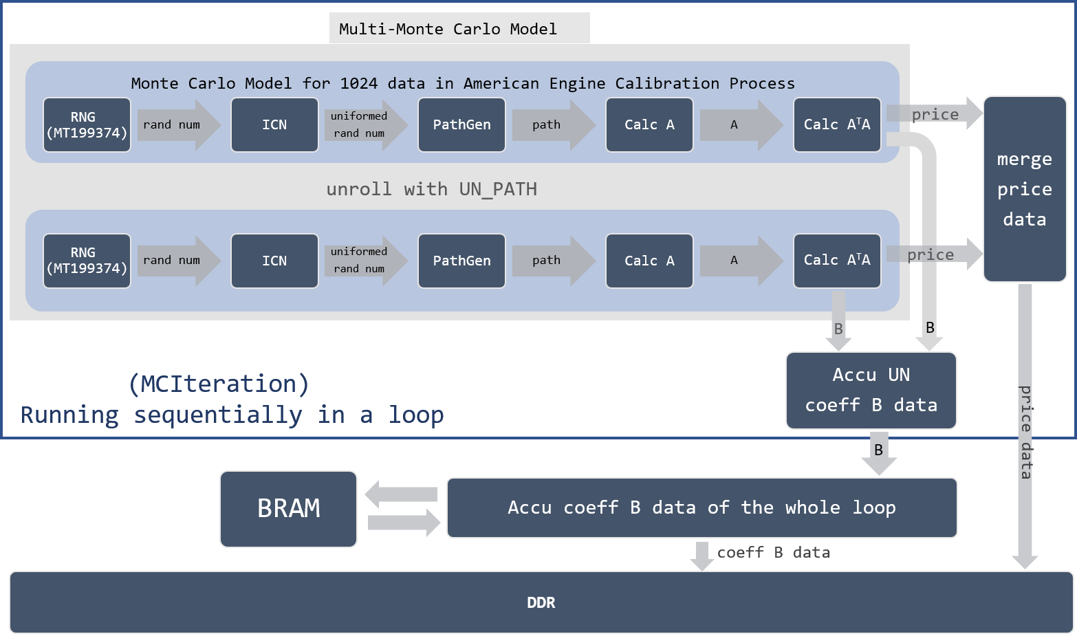
We denote the process from RNG to generate matrix data \(B\) and exercise price for each timestep \(t\) as a Monte-Carlo-Model (MCM) in American Option Calibration Process. Each MCM process 1024 data. With a template parameter UN_PATH, more pieces of MCM can be instanced when hardware resources available.
To connect multiple MCM data, two merger blocks are created: one for merge price data, one for merge matrix \(B\). Meanwhile, to guarantee all calibration path data can be executed in a loop when there is not enough MCM available, a soft-layer Merger that accumulates all elements of \(B\) data is employed. Since these intermediate data need to be accumulated multiple times, a BRAM is used to save and load them.
- Once we get the matrix \(B\), the singular matrix \(\Sigma\) of \(B\) could be obtained by SVD (Singular Value Decomposition).
- Thereafter, use Least-Squares to calculated the coefficients by modifying Equation (3) to:
Until now, matrix \(B\) and vector \(y\) are known, coefficients \(x\) could be calculated.
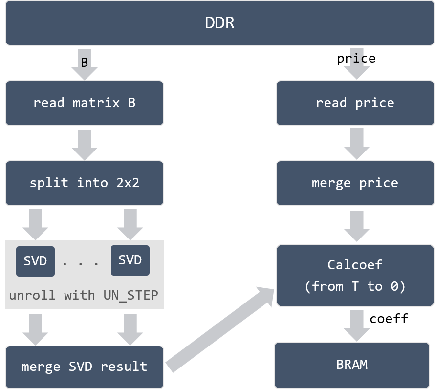
The implementation of step 3 and steps 4 is shown in Figure 12. Because step 2 generates matrix \(B\) and price data \(y\) from timesteps \(0\) to \(T\). Step 3 processes these data in the backward direction, from timesteps \(T\) to \(0\). Considering the amount of data, 4096*timesteps*8*sizeof(DT) and 9*timesteps*8*sizeof(DT), it is impossible to store all the data on FPGA. In the implementation, DDR/HBM memory is used to save these data. Correspondingly, DDR data read/write modules are added to the design.
Besides, notice that since SVD is purely computing dependent, which is pretty slow in the design. Therefore, a template parameter UN_STEP is added to speed up the SVD calculation process.
Note
It is worth mentioning that 4096 is only the default calibrate sample/path size. This number may change by customers’ demands. However, the size must be a multiple of 1024.
Pricing Process
MCAmericanEnginePricing
The theory of the pricing process is actually already introduced in the Theory Section. Similar to the European option engine, mcSimulation framework is employed. Compared to the European option engine, the difference is that it needs to calculate the optimal exercise at all time steps. The detailed implementation process of American engine is drawn as Figure Figure 13 shows.
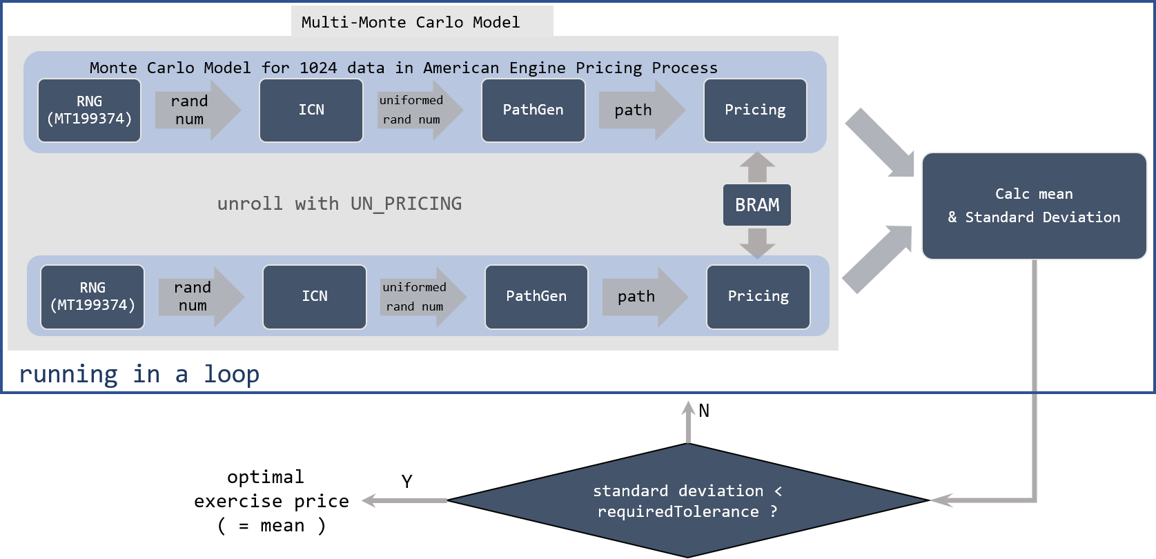
- Generate uniform random numbers with Mersenne Twister UNiform MT19937 Random Number Generator (RNG) followed by Inverse Cumulative Normal (ICN) uniform random numbers. Thereafter, generate independent stock paths with the uniform random numbers and Black-Sholes path generator.
- Refer to Equation (2), calculate the exercise price at time step \(T\) by utilizing the calculated coefficients \(x\).
- Calculate the exercise price for previous time steps \(t\), and take the max exercise price by comparing the immediate exercise price with the held price value (maximum value for time steps \(t+1\)).
- Continue the process, until time step \(t\) equals 0, optimal exercise price and the standard deviation is obtained.
- Check if the standard deviation is smaller than the required tolerance defined by customers. If not, repeat step 1-4, until the final optimal exercise price is obtained.
Caution
Notice that the pricing module also supports another approach of ending pricing process, which utilizes the input parameter requiredSamples. When the requiredSamples are processed, we assume the output mean result is the final optimal exercise price. This mode is also supported in the American Option Pricing Engine. And the figure above only illustrates the ending approach with the required tolerance.
Note
In the figure, BRAM is used to load coefficients data that calculated from the calibration process. Here may use BRAM or DDR, it depends on the amount of data that need to be stored beforehand. The reason that coefficients data cannot be streamed is that the multi-Monte-Carlo process in pricing always needs to execute multiple times. Each time execution, these need to be loaded. Thus, it is impossible to use hls::stream.
MCAmericanEngine APIs
In our library, the MCAmerican Option Pricing with Monte Carlo simulation is provided as an API MCAmericanEngine(). However, due to external memory usage on DDR/HBM and avoiding the designed hardware cross-SLR placed and routed. The American engine option supports two modes:
- single API version: use one API to run the whole American option
- three APIs version: three APIs/kernels are provided, connecting them on the host side to compose the overall design.
The boundary between them is external memory access. For the calibration process, two APIs are provided. Calibration step 1 and 2 are wrapped as one kernel, namely, MCAmericanEnginePreSamples. Step 3 and step 4 compose another kernel MCAmericanEngineCalibrate. And pricing process as another kernel MCAmericanEnginePricing in this library. Because the pricing process is separated as a kernel, the data exchange between the calibration and pricing process may not through the BRAM any more. Thus, in the implementation, DDR/HBM is used as the coefficients data storage memory.
With the three kernels, the kernel level pipeline by shortening the overall execution time could be achieved. However, employing kernel level pipeline requires a complex schedule from the host code side. An illustration of connection 3 kernels as a complete system is given in this part, which can be seen in Figure 14. Price data and \(B\) matrix data are the outputs from kernel MCAmericanEnginePreSamples. For each timestep, path number (default 4096) price data B and x matrix data (a number of 9) need to be saved to DDR or HBM memory.
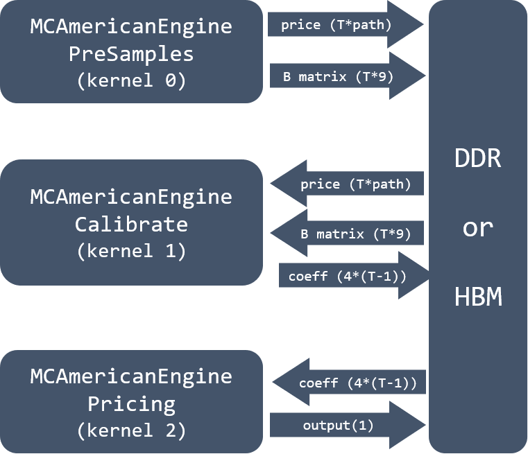
Kernel 1 MCAmericanEngineCalibrate reads price data \(y\) and matrix data \(B\) from external memory and outputs coefficients to DDR/HBM. The last kernel MCAmericanEnginePricing reads coefficients data from DDR/HBM and saves the final output optimal exercise price to DDR/HBM.
Hint
Why the number of matrix B is 9 in DDR/HBM?
The matrix \(A\) is 4096 * 4 for each timestep when the path number is 4096 (default). The size of its transform matrix \(A^T\) is 4 * 4096. So, the size of matrix \(B\) is 4 * 4. However, some elements in \(B\) are the same, and 9 can represent all 16 data. More precisely, assuming
It is evident that some elements are the same. After removing duplicated elements, the following 9 elements of \(B\) are stored to DDR/HBM each timestep:
Caution
The architecture illustrated above is only an example design. In fact, multiple numbers of kernels, each with a different unroll number (UN) may be deployed. The number of kernels that can be instanced in design depends on the resource/size of the FPGA.