Internal Design of Asian Option Pricing Engine
Overview
The Asian option pricing engine uses Monte Carlo Simulation to estimate the value of the Asian option. Here, we assume the process of asset pricing applies to Black-Scholes process.
Asian Option is kind of exotic option. The payoff is path dependent and it is dependent on the average price of underlying asset over the settled period of time \(T\).
The payoff of Asian options is determined by the arithmetic or geometric average underlying price over some pre-set period of time. This is different from the case of usual European Option and American Option, where the payoff of the option depends on the price of the underlying at exercise. One advantage of Asian option is the relative cost of Asian option compared to American options. Because of the averaging feature, Asian options are typically cheaper than American options.
The average price of underlying asset could be used as strike price or the underlying settlement price at the expiry time. When the average price of underlying asset is used as the underlying settlement price at the expiry time, the payoff is calculated as follows:
payoff of put option = \(\max(0, K - A(T))\)
payoff of call option = \(\max(0, A(T) - K)\)
When the average price of underlying asset is used as the strike price at the expiry time, the payoff is calculated as follows:
payoff of put option = \(\max(0, A(T) - S_T)\)
payoff of call option = \(\max(0, S_T - A(T))\)
Where \(T\) is the time of maturity, \(A(T)\) is the average price of asset during time \(T\), \(K\) is the fixed strike, \(S_T\) is the price of underlying asset at maturity.
The average could be arithmetic or geometric, which is configurable. \(N\) is the number of discrete steps from \(0\) to \(T\).
Arithmetic average: \(A(T) = \frac{\sum_{i=0}^N S_i}{N}\)
Geometric average: \(A(T) = \sqrt[n]{\prod_{i=0}^N S_i}\)
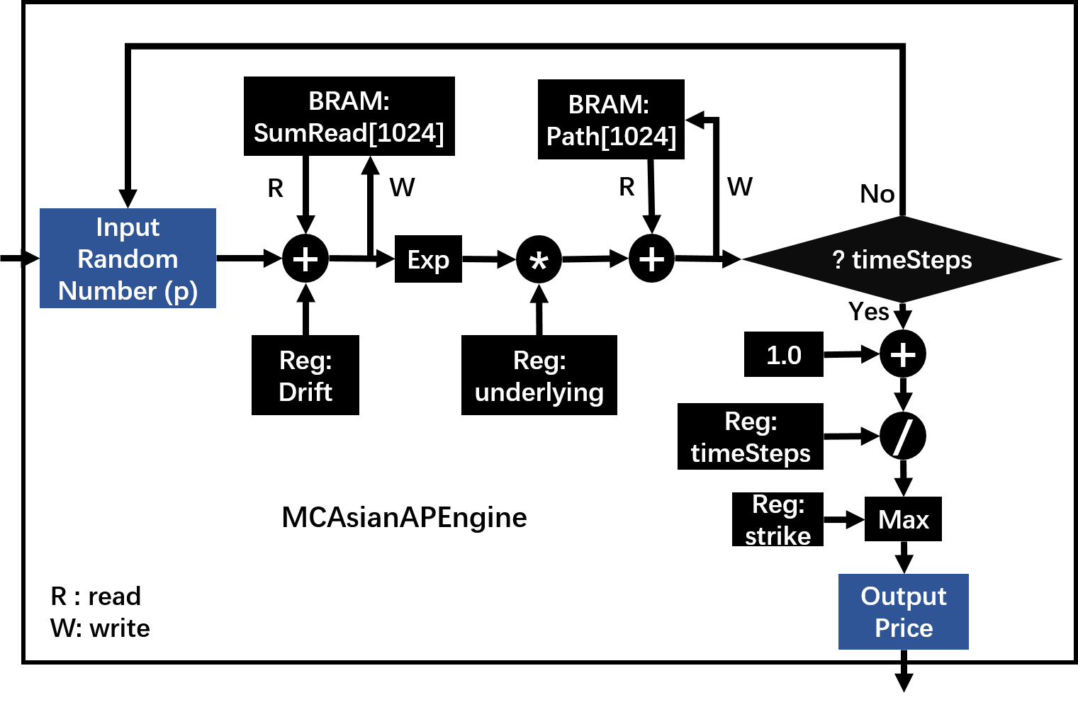
MCAsianAPEngine
The pricing process of Asian Arithmetic Pricing engine is as follows:
- Generate independent stock paths by using Mersenne Twister Uniform MT19937 Random Number Generator (RNG) followed by Inverse Cumulative Normal Uniform Random Numbers.
- Start at \(t = 0\) and calculate the stock price of each path firstly in order to achieve initiation interval (II) = 1.
- Calculate arithmetic average and geometric average value of each path.
- Calculate the payoff difference of arithmetic average price and geometric average price.
- Calculate the payoff off of geometric average price \(Payoff_{ref}\) based on analytical method.
- Payoff of average pricing is \(Payoff = Payoff_{ref} + Payoff_{gap}\)
The pricing architecture on FPGA can be shown as the following figure:
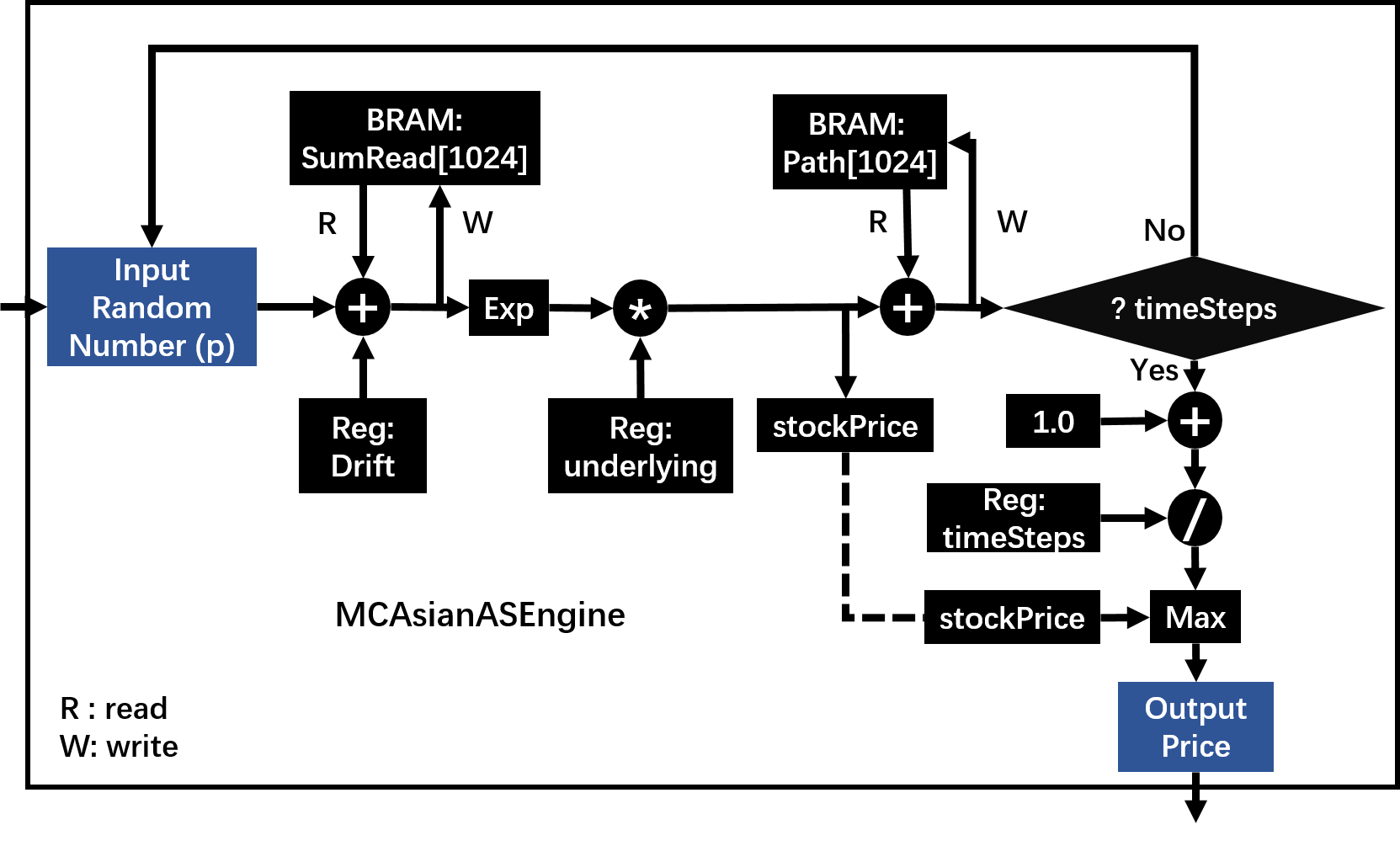
MCAsianASEngine
The pricing process of Asian Arithmetic Strike engine is as follows:
- Generate independent stock paths by using Mersenne Twister Uniform MT19937 Random Number Generator (RNG) followed by Inverse Cumulative Normal Uniform Random Numbers.
- Start at \(t = 0\) and calculate the stock price of each path firstly in order to achieve II = 1.
- Accumulate the sum of lognormal stock price using the following analytical solution.
where \(M\) is the total timesteps, \(dt\) is the time interval 4. Calculate the final payoff by taking the strike price \(Strike_t\) as the previous arithmetic average price \(\frac{\sum_{j=0}^i S_j}{M}\).
The pricing architecture on FPGA can be shown as the following figure:
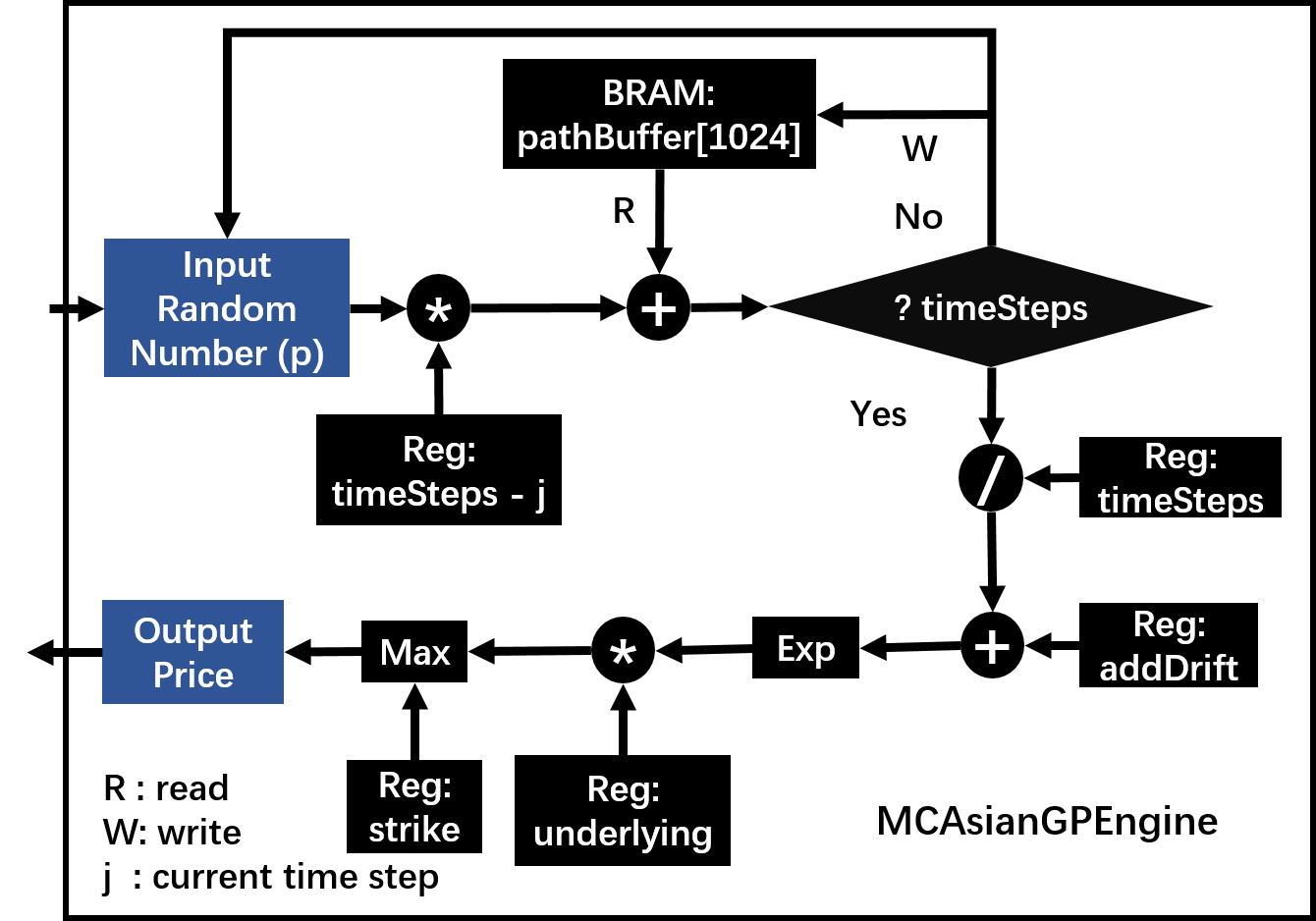
MCAsianGPEngine
The pricing process of Asian Geometric Pricing engine is as follows:
- Generate independent stock paths by using Mersenne Twister Uniform MT19937 Random Number Generator (RNG) followed by Inverse Cumulative Normal Uniform Random Numbers.
- Start at \(t = 0\) and calculate the stock price of each path firstly in order to achieve II = 1.
- Transfer the geometric average of stock price to sum of lognormal stock price.
- Accumulate the sum of lognormal stock price using the following analytical solution.
- Calculate the final payoff by using a fixed strike price.
The pricing architecture on FPGA can be shown as the following figure:
Note
The 3 figures above shows the pricing part of McAsianAPEngine, McAsianASEngine and McAsianGPEngine respectively; the other parts, for example, PathGenerator, MCSimulation and other modules, are the same as in MCEuropeanEngine.
Profiling
The hardware resources are listed in Table 4. The Arithmetic and Geometric Asian Engines demand similar amount of resources.
| Engines | BRAM | DSP | Register | LUT | Latency | clock period(ns) |
| McAsianArithmeticAPEngine | 12 | 59 | 24664 | 26826 | 53276 | 3.423 |
| McAsianArithmeticASEngine | 12 | 65 | 26683 | 29362 | 53196 | 3.423 |
| McAsianGeometricAPEngine | 10 | 61 | 24626 | 26657 | 53222 | 3.423 |
Table 5 shows the performance improvement in comparison with CPU-based Quantlib result (Tolerance = 0.02)
| Engines | McAsianAPEngine | McAsianASEngine | McAsianGPEngine |
| SampNum | 25951 | 33642 | 46805 |
| CPU result | 1.98441 | 3.10669 | 3.28924 |
| CPU Execution time (us) | 224911 | 310856 | 601068 |
| FPGA result | 1.89144 | 3.0866 | 3.26228 |
| FPGA Kernel Execution time (us) | 563.05 | 734.42 | 830.130 |
| FPGA SampNum | 28672 | 34816 | 49152 |
| FPGA E2E Execution time (ms) | 1 | 1 | 1 |
| Number of MCM | 2 | 2 | 4 |
Table 6 shows the max performance of McAsianEngines in one SLR of Xilinx xcu250-figd2104-2L-e (Vivado report).
| Engines | BRAM | DSP | Register | LUT | Latency |
|
Max Unroll Num |
| McAsianArithmeticAPEngine | 192 | 749 | 246325 | 205626 | 54056 | 300 | 16 |
| McAsianArithmeticASEngine | 192 | 755 | 247524 | 207476 | 54109 | 300 | 16 |
| McAsianGeometricAPEngine | 160 | 781 | 242927 | 200106 | 54002 | 300 | 16 |