Internal Design of LIBOR Market Model
Overview
Thie LIBOR Market Model (LMM) framework, also known as Brace Gatarek Musiela model (BGM) is a financial model of interest rates. The quantities that are modeled are a set of forward rates (also called forward LIBORs) unlike the HJM framework which uses instantaneous forward rates. The main advantage of this model over HJM is that the forward rates are observable in the market and their volatilities are naturally linked to traded contracts. Our implementation is modelled by a lognormal process and solved by Monte-Carlo simulation.
Design Structure
For a given tenor structure \(T_0,T_1,...,T_n\) evenly spaced with \(\tau = T_{i+1} - T_i, \forall i=1,...,n\), and a number of factors \(F\), we evolve the LIBOR rates for all \(n\) maturities with the following stochastic equation:
Where \(\sigma_i(t)\) are calibrated volatilities, \(dW_i\) is a Brownian motion scaled by the pseudo-sqrt of the correlations matrix and \(\mu_i(t)\) is the drift defined in terms of the volatilities and correlations between tenors:
Calibration of the Model
In order to correctly use the model, the tenor correlations and volatilities must be calibrated to market data. The correlation and volatilities matrix is an input to the model and can potentially acept any user-defined data, but we also provide some common parametric functions that can generate suitable calibrations.
Correlation calibration
The instantaneous tenor correlation matrix \(\rho\) is an input to the LMM framework. These correlation matrices should be in the form of symmetric, positive and monotonically decreasing, as that would be expected from real correlations from the market data. Our implementation provides a family of parametric correlation functions that can be chosen. In order to avoid noise in calibration it is recommended to use as few parameters as possible. With that in mind the following functions are available:
- One-parametric instantaneous correlation. User needs to specify \(\beta\) with a value \(0 < \beta <= 1\):
- Two-parametric instantaneous correlation. User needs to specify \(\beta_0,\beta_1\) with values \(0<\beta_0\beta_1<=1\):
Once a correlation matrix is generated, a Principal Component Analysis will be performed to reduce the dimensionality of the data to \(F\) factors, in order to calculate the reduced factor correlation matrix (\(\bar{\rho}\)) and the pseudo-sqrt of the correlation matrix (\(\eta\)) used in the LMM framework. The dimensionality reduction is applied as follows:
- Calculate the \(F\) factors loadings matrix of the correlation matrix \(\rho\):
- The \(\eta\) matrix is the loadings matrix normalised by the standard deviation (sqrt of the covariance matrix’s diagonal):
- From matrix \(\eta\), we can reduce the dimensionality of the original data set to obtain \(\tilde{\rho}\):
Volatility Calibration
For the calibration of volatilities, we provide a volatily generator with values that can be bootstrapped from a vector of caplet implied volatitilies obtained via the Black76 model. Implied volatitilies are the values that, when put into the Black formula, return the price that the option currently has in the market. It is market practise to quote the price of a caplet for a tenor \(T_i\) by just their implied volatily and not the actual price. Our implementation uses a calibration formula that will bootstrap the implied volatilities into a stationary piecewise constant volatility vectors used by the LMM. This implies that the calculated volatilities are identical for all fixed times to maturity and they change over time as time to maturity changes \(\gamma(t,T) = \gamma(T - t)\)
In order to calibrate the model, our provided function we take a vector of implied caplet volatilities \(\hat{\sigma}_i\) as input and will generate the volatility matrix as follows:
Since as we advance \(t\) up to maturity time each tenor expires, our generated volatilities will take the form of a lower triangular matrix:
| \([0,T_0]\) | \((T_0,T_1]\) | \((T_1,T_2]\) | … | \((T_{n-2},T_{n-1}]\) | \((T_{n-1},T_n]\) | |
| \(L_1(t)\) | \(\sigma_1(T_0)\) | expired | expired | … | expired | expired |
| \(L_2(t)\) | \(\sigma_2(T_0)\) | \(\sigma_1(T_1)\) | expired | … | expired | expired |
| … | … | … | … | … | … | … |
| \(L_n(t)\) | \(\sigma_n(T_0)\) | \(\sigma_{n-1}(T_1)\) | \(\sigma_{n-2}(T_2)\) | … | \(\sigma_1(T_n)\) | expired |
Pricing Algorithms
Currently we support several choices for pricing algorithms by default, but the model can accept any custom implementation as a parameter. Each pricer will consume one generated LIBOR rates path and output a price, which will be accumulated and averaged out to provide the Monte-Carlo solution.
Cap Pricing
A cap is a basket of caplets, where all caplets have the same strike (caprate). Each caplet will have a payoff at time \(T_1, T_2, ..., T_n\). The price of the cap will be the sum of all the caplets. The pricing of caps with the LMM framework is interesting because we can use it to validate the model and the calibrations by comparing the output of the MonteCarlo simulation with the output from the analytical Black76 model. Once we are satisfied with the results from the model, we can use the same parameters to compute the pricing of other options that don’t have analytical formulas.
The general formula for the price of a cap with notional \(N\) and caprate \(K\) is given by:
Analytically, we can use the Black76 formula to calculate the price of a caplet with:
With the LIBOR market model, we can calculate the price of a caplet with the following formula:
After generating enough paths, the average of all Cap prices with the LMM will converge to the value from the Black76 formula provided the model is correctly calibrated.
Ratchet Floater Pricing
A ratchet floater is a path dependent interest rate product. This option is a good example for the use of the LIBOR market model, since no analytic formula exists. At each time \(T_i, i > 0\), the ratchet pays a coupon amount \(c_i\). The ratchet floater price is the sum of all coupons.
For a ratchet floater with notional \(N\), constant spreads \(X\) and \(Y\) and fixed cap \(\alpha\) the price can be calculated with:
This means that the coupon \(c_i\) is at least as much as the previous coupon amount, but no more than the previous coupon plus a fixed constant \(N\alpha\)
Ratchet Cap Pricing
Ratchet caps have a similar structure as standard caps. The main difference is that while caps have a fixed caprate for every caplet, for ratchet caps we will have a variable caprate dependent on earlier LIBOR resets for every ratchet caplet plus a spread.
The price of a ratchet cap with notional \(N\), spread \(s\) and initial spread \(\kappa_0\) is given by the following formula:
Internal Architecture
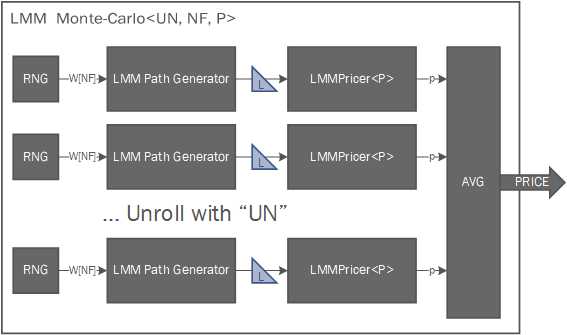
The internal framework implementation allows to easely parallelise the generation and pricing of LIBOR rates matrices by modifying the UN parameter. Each unrolled implementation will contain a RNG sequence generator for \(F\) uncorrelated factors, a LMM path generator and a copy of the chosen path pricer. Since the calibration data (\(\eta,\bar{\rho},\sigma\)) is computed once and then read only, each MonteCarlo module will also contain a copy of the accessed elements of those matrices.
The path generator will compute a set of LIBOR rates, which are of the form of a lower triangular matrix, with the following process:
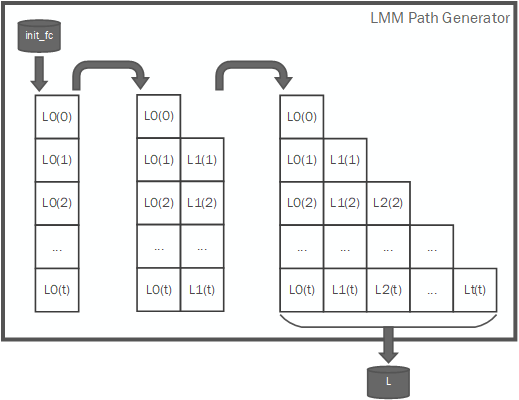
Each LIBOR rates path matrix will be fed via an HLS stream into the path pricer in a strided pattern: First the \(L_0\) column, from \(T_0\) to \(T_n\). Then the \(L_1\) column and so on.
It is responsibility of the path pricer to compute the option price and to consume the all the data fed from the path generator.
The full implementation of the LIBOR Market Model framework has the following architecture: