Random Number Generator
Overview
Random Number Generator (RNG) is one of the core utilities needed by Monte Carlo Simulation. We provide RNGs that generate uniform distribution and normal distribution. The detailed supported RNGs are listed below.
| RNG name | Distribution generated | DataType supported | Underlying Algorithm |
|---|---|---|---|
| MT19937 | Uniform Distribution in (0,1) | float, double | Mersenne Twister (MT19937) |
| MT2203 | Uniform Distribution in (0,1) | float, double | Mersenne Twister (MT2203) |
| MT19937IcnRng | Normal Distribution N(0,1) | float, double | Inverse CDF Transformation |
| MT2203IcnRng | Normal Distribution N(0,1) | float, double | Inverse CDF Transformation |
| MT19937BoxMullerNomralRng | Normal Distribution N(0,1) | float, double | Box Muller Transformation |
| MultiVariateNormalRng | Multi Variate Normal Distribution | float, double | Cholesky Decomposition |
Uniform Distributed Random Number Generator
Uniform Distributed Random Number Generator is the foundation of all RNGs. In this implementation, we use the Mersenne Twister Algorithm (MT19937 and MT2203) as the underlying algorithm.
Reference: Mersenne Twister.
Algorithm
The basic element of Mersenne Twister (MT) Algorithm is vector, a \(w\) bits unsigned integer. The MT Algorithm generates a sequence of vectors, which are considered to be uniform distributed in \((0, 2^w - 1)\). These vectors could be mapped to (0,1) after dividing by \(2^w\).
The basic algorithm is composed of two parts. First part is an iterative formula as shown below:
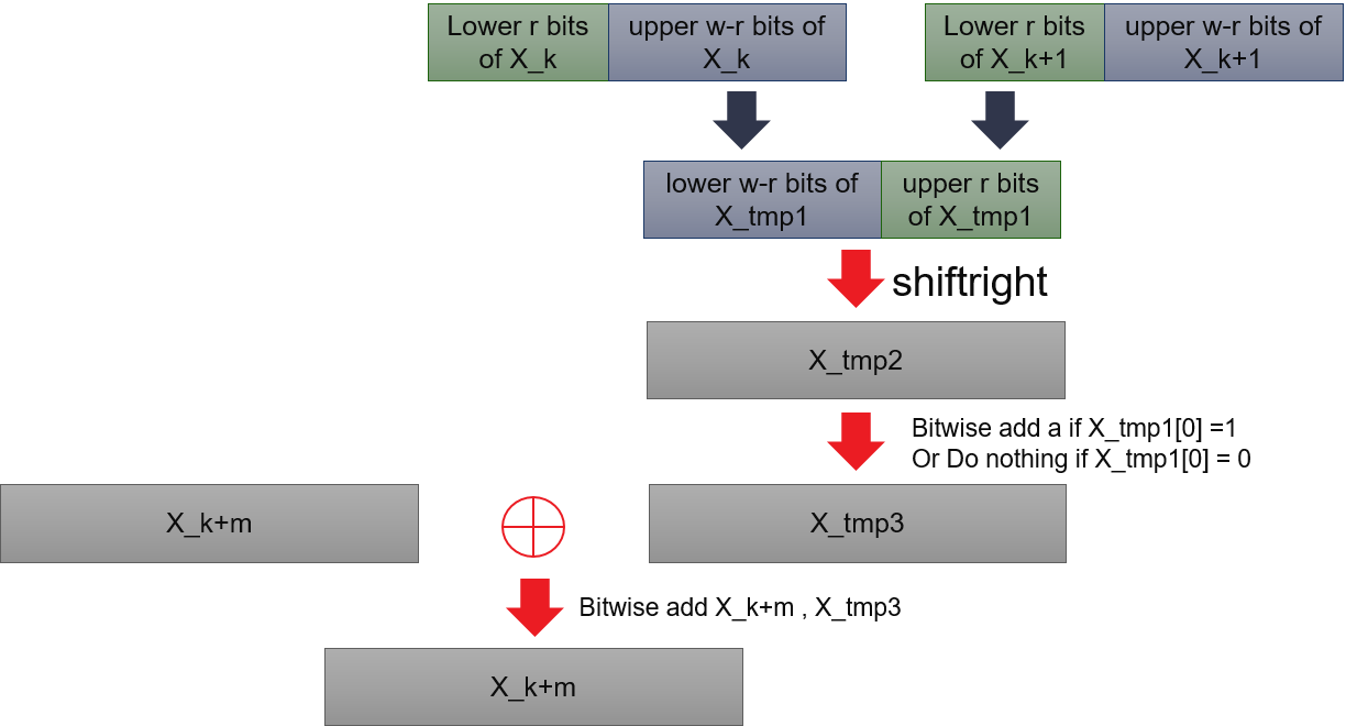
Where \(X_{k + n}\) denotes the \(k\), \(X_1\),…, \(X_{n - 1}\) as initial vectors. \(X_{k}^u\) means the upper \(w - r\) bits of \(X_{k}\), \(X_{k + 1}^u\) means the lower \(r\) bits of \(X_{k + 1}\). \((X_{k}^u|X_{k+1}^l)\) is just combination of upper \(w - r\) bits of \(X_{k}\) and lower \(r\) bits of \(X_{k + 1}\). \(\bigoplus\) is bitwise addition. The multiplication of \(A\) could be done by bits operations:
Where \(a\) is a constant vector.
The second part is tempering, which consists of four steps below.
Where \(u\), \(s\), \(t\), and \(l\) are constant parameters indicate shift length, \(b\) and \(c\) are two const vectors.
A combination of \(w\), \(n\), \(r\), \(m\), \(u\), \(s\), \(t\), \(l\), \(a\), \(b\), \(c\) determines a variation of Mersenne Twister. Only a limited combination could work.
Implementation Details
The optimization happens in the first part. We don’t store all history of vectors generated, only the last \(n\) vectors. We use a circular queue in BRAMs to store these values. Depth of BRAM is set to be least 2’s power that larger than n. This will make the calculation of the address simpler. By keeping and updating the address of the starting vector, we can always calculate the address of vectors we need to access.
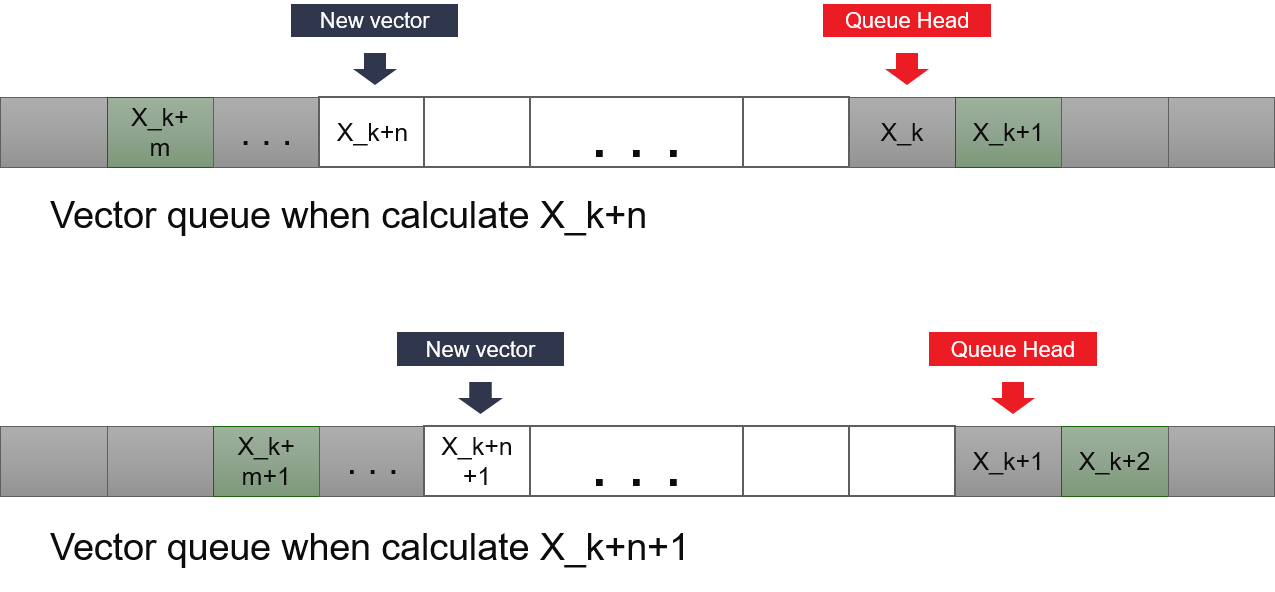
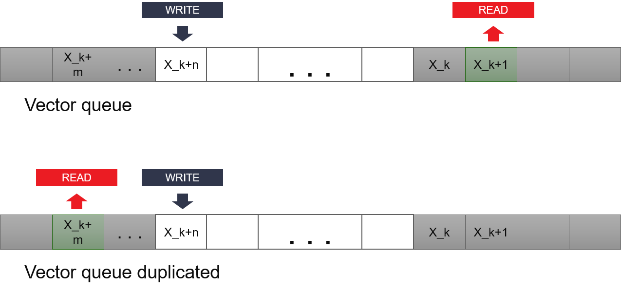
To generate k-th vector, we need 3 read ops, for \(X_{k}\), \(X_{k + 1}\) and \(X_{k + m}\). In the next iteration, we need to read \(X_{k + 1}\), \(X_{k + 2}\) and \(X_{k + m + 1}\). This means we only need to read \(X_{k + 2}\) and \(X_{k + m + 1}\), since we could save \(X_{k + 1}\) in a register. So, we need 2 read accesses at different vectors and 1 write access for generating the new vector. Since BRAM only allows 2 read or write accesses at a single cycle, it’s not capable of generating the new vector at each clock cycle. In the implementation, we copy the identical vectors to different BRAMs, and each of them provides sufficient read or write access port.
Normal Distributed Random Number Generator (NRNG)
NRNG is the most useful RNG in Monte Carlo Simulation. We provide two kinds of NRNG: Inverse Cumulative Distributed Function based NRNG and Box-Muller transformation based NRNG.
Inverse cumulative distribution transformation based RNG
For a certain distribution of random variable \(Z\), it has a corresponding cumulative distribution function \(\Psi(x)\). This function measures the probability that \(Z < x\). Since \(\Psi(x)\) is monotonically increasing function, it has an inverse function \(\Psi^{-1}(x)\). It is mathematically approved that for uniform-distributed random variable \(U\) in range (0, 1), \(\Psi^{-1}(U)\) is also a random variable and its cumulative distribution function is \(\Psi(x)\).
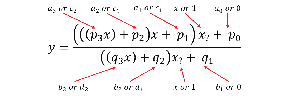
We have two versions of Inverse Cumulative Distribution Function (ICDF) with the data type of float or double, details of algorithms could be found from reference papers. Both of them use fractional polynomial approximation method. They both have two branches for value from different input range and they share similar logics. To save DSPs, we combined the two branches and manually binding calculation to the same hardware resource to get the same performance and accuracy. Take ICDF with float data type as an example, the basic approximation formula is (main fractional polynomial approximation part, not all) shown as below:
Although these two conditions have different formulas, they can merge into one formula with parameters configured by which range that \(x\) belongs to. As shown in the diagram below, if parameters took the value at left, it would become the first formula above. If at right, it would become the second formula above.
Box-Muller transformation based NRNG
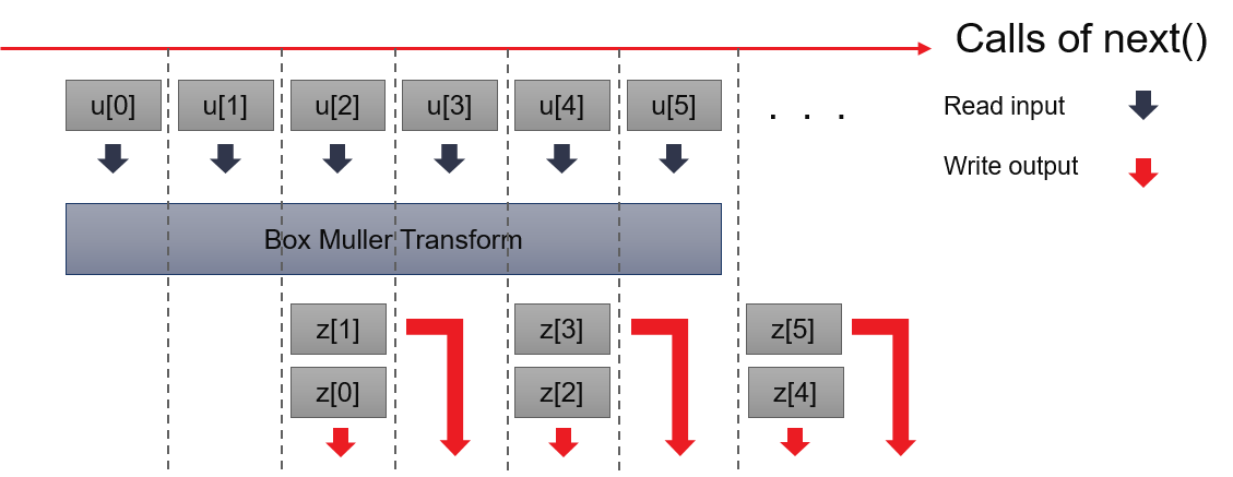
Box-Muller transformation takes two uniformed distributed random numbers to generate two normal-distributed random number. Although it is an efficient method, it could not hold certain algebra characteristics of input uniformed distributed random number serials, especially when we need NRNG in low-discrepancy serials. It’s not the first choice of NRNG in the current stage.
To smooth output, Box-Muller implementation takes 1 uniformed random number at each call of next(), outputs 1 normal distributed random number which is already generated and cached. When 2 inputs have been cached, it performs Box-Muller transformation above and generates the next two normal-distributed random numbers.
Multi Variate Normal Distribution RNG
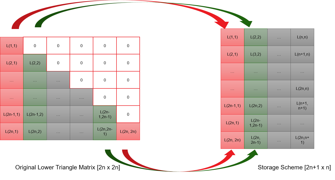
Multi-variate normal distribution RNG output N random variates. Each variate’s distribution is N(0, 1), and these variates have a certain correlation. To generate such variates, this RNG needs to set up the lower triangle matrix first, which is the result of the Cholesky decomposition of the correlation matrix. This implementation supports an even number of variate which is 2N. Instead of storing a 2N-by-2N matrix, we only store the N*(2N+1) non-zero elements. The storage scheme is as below. This RNG needs to pre-calculate a certain number of random numbers before it can output the right random number.
Put the storage scheme aside, the basic working principle is using one underlying random number generator to produce several independent random numbers. Every 2N independent random numbers compose a vector. By multiplying this vector with the lower triangle matrix, we get the result vector. Elements of result vector are multi-variate normal distribution random numbers, which have the pre-set correlation.