Principal Component Analysis
Overview
Principal Component Analysis (PCA) is a statistical procedure that uses an orthogonal transformation to convert a set of observations of possibly correlated variables into a set of linearly uncorrelated variables called Principal Components.
In quantitative finance, PCA can be directly applied to risk management of interest rate derivative portfolios. It helps reducing the complexity of swap tradings from a function of 30-500 market instruments to, usually, just 3 or 4, which can represent the interest rate paths on a macro basis.
Implementation
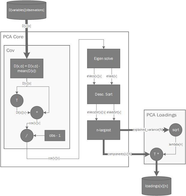
The PCA of N components of an m-by-n matrix A is given by the following process:
- Calculate the covariance matrix of A
- Solve n-by-n covariance matrix for its n-by-n eigen-vectors (\(V\)) and n eigen-values (\(D\))
- Sort the eigen-values from largest to smallest and then select the top \(N\) eigen-values and their corresponding eigen-vectors.
Once the process is completed there are several outputs available from the library:
- ExplainedVariance: This is a vector N wide which corresponds to the selected sorted eigen-values.
- Components: These are the N eigen-vectors associated with the selected eigen-values of the original matrix.
- LoadingsMatrix: The loadings matrix represent the weigths associated to each original variable when calculating the principal components. It can be computed as follows:
Note
Due to the arbitrary sign of eigen-vectors, them being implementation dependent, calculations of the loadings matrix could return inverted values in a non-deterministic way. To avoid that, we use the same convention as matlab, where the sign for the first element of each eigen-vector must be positive, multiplying the whole vector by \(-1\) otherwise.
Below is a diagram of the internal implementation of PCA:
