Interpolation
Overview
In the mathematics, interpolation can be viewed as an estimate, a method of constructing new data points within a discrete set of known data points. Here a variety of interpolation methods are implemented, including linear interpolation, cubic interpolation, and bicubic interpolation.
Algorithm & Implementation
Linear interpolation
There are two points \(A\left ( x_{A},y_{A} \right )\) and \(B\left ( x_{B},y_{B} \right )\) in the two-dimensional coordinate system. The linear interpolation calculates the value of :math: xepsilon left [ x_{B}, x_{B} right ] on the AB line. Its expression is:
The implementation is very simple and not elaborated here. For more information, please check out source code and `linear`_.
.._`linear`: https://en.wikipedia.org/wiki/Linear_interpolation
Cubic interpolation
The cubic interpolation algorithm is in `cubic`_, and The cubic interpolation implementation is in source code.
.._`cubic`: https://www.paulinternet.nl/?page=bicubic
Bicubic spline interpolation
The bicubic spline interpolation is an extension of cubic interpolation for interpolating data points on a two-dimensional regular grid. For more algorithm details, please see `bicubic`_. Its implementation is essential to perform interpolation according to the x-direction, and then to interpolate in the y-direction. Then the desired result can be obtained.
.._`bicubic`: https://en.wikipedia.org/wiki/Bicubic_interpolation
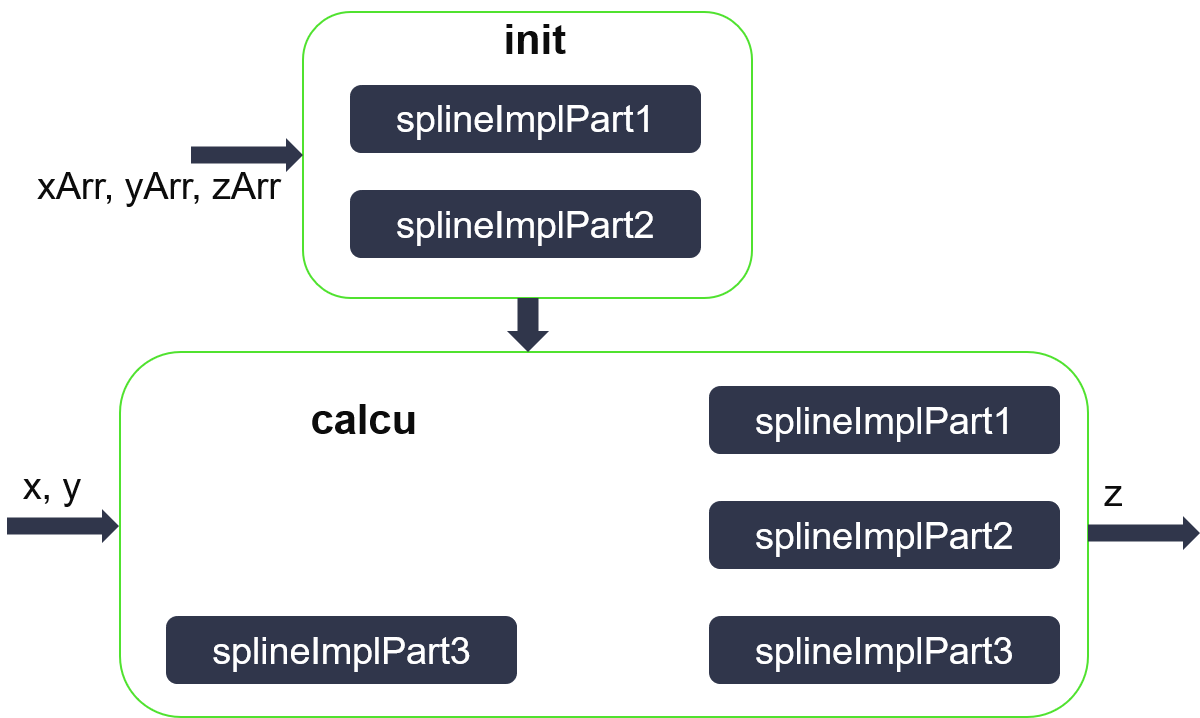
As shown in the figure below, the interpolation implementation includes 2 parts: init and calcu.
- The init mainly implements parameter pre-processing and some functions of cubic spline interpolation in x-direction.
- The calcu completes cubic spline interpolation in the x-direction according to the input x and results of the init, and then completes cubic spline interpolation in the y-direction according to the obtained result and the input y to obtain an output result.
