Singular Value Decomposition (SVD)¶

Overview¶

The singular value decomposition (SVD) is a very useful technique for dealing with general dense matrix problems. Recent years, SVD has become a computationally viable tool for solving a wide variety of problems raised in many practical applications, such as least-squares data fitting, image compression, facial recognition, principal component analysis, latent semantic analysis, and computing the 2-norm, condition number, and numerical rank of a matrix.

For more information, please refer to SVD.

Theory¶

The SVD of an m-by-n matrix A is given by

\[A = U \Sigma V^T (A = U \Sigma V^H \, in \, the \, complex \, case)\]

where \(U\) and \(V\) are orthogonal (unitary) matrix and \(\Sigma\) is an m-by-n matrix with real diagonal elements.

Theoretically, the SVD can be characterized by the fact that the singular values are the square roots of eigenvalues of \(A^TA\), the columns of \(V\) are the corresponding eigenvectors, and the columns of \(U\) are the eigenvectors of \(AA^T\), assuming distinct singular values. The approximation can simplify the general m-by-n matrix SVD problem to a general symmetric matrix SVD problem. Due to the roundoff errors in the formulation of \(AA^T\) and \(A^TA\), the accuracy is influenced slightly, but if we don’t need a high-accuracy, the approximation can largely reduce the complexity of calculation.

There are two dominant categories of SVD algorithms for dense matrix: bidiagonalization methods and Jacobi methods. The classical bidiagonalization method is a long sequential calculation, FPGA has no advantage in that case. In contrast, Jacobi methods apply plane rotations to the entire matrix A. Two-sided Jacobi methods iteratively apply rotations on both sides of matrix A to bring it to diagonal form, while one-sided Hestenes Jacobi methods apply rotations on one side to orthogonalize the columns of matrix A and bring \(A^TA\) to diagonal form. While Jacobi methods are often slower than bidiagonalization methods, they have better potential in unrolling and pipelining.

Jacobi Methods¶

Jacobi uses a sequence of plane rotations to reduce a symmetric matrix A to a diagonal matrix

\[A_{0} = A, \> A_{k+1} = J_{k}^{T}A_{k}J_{k}, \> A_{k} \rightarrow \Sigma \> as \> k \rightarrow \infty\]

Each plane rotation, \(J_{k} = J_{k}(i, j, \theta)\), now called a Jacobi or Givens rotation

(1)¶\[\begin{split}\begin{equation} J_{k}(i, j, \theta)=\begin{vmatrix} I &\, & & & \\ \, &\,c & &s & \\ \, &\, &I & & \\ \, &-s & &c & \\ & &\, & & &I \end{vmatrix} \end{equation}\end{split}\]

where \(c=cos \theta\) and \(s=sin \theta\). The angle \(\theta\) is chosen to eliminate the pair \(a_{ij}\), \(a_{ji}\) by applying \(J(i,j, \theta )\) on the left and right of \(A\), which can be viewed as the 2x2 eigenvalue problem

\[\begin{split}\begin{equation} \hat{J}_{(k)}^{T} \hat{A}_{(k)} \hat{J}_{(k)}= \begin{vmatrix} \, c &s \\ -s &c \end{vmatrix}^{T} \begin{vmatrix} a_{ii} &a_{ij} \\ a_{ji} &a_{jj} \end{vmatrix} \begin{vmatrix} d_{ii} &0 \\ 0 &d_{jj} \end{vmatrix}= \hat{A}_{(k+1)} \end{equation}\end{split}\]

where \(\hat{A}\) is a 2X2 submatrix of matrix A. After the Givens rotations of the whole matrix A, the off-diagonal value of A will be reduced after 5-10 times iteration of the process.

Implementation¶

SVD workflow:¶

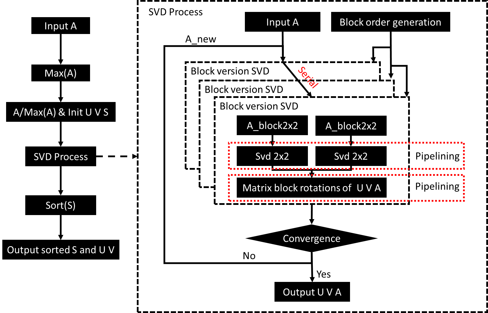
The input parameters for the 4x4 SVD function is the 4x4 matrix \(A\), and the output matrices are \(U\), \(V\), and \(\Sigma\) respectively. As shown in the above figure, the SVD process has 4 main steps:

Find the max value of matrix \(A\);
Divide all member of A by \(max(A)\) and initiate \(U\), \(\Sigma\), \(V\);
The iterative process of Jacobi SVD;
Sort matrix \(S\), and change \(U\) and \(V\);

The iterative process of Jacobi SVD is the core function. Firstly, the matrix \(A\) will be divided into 2x3 (= \(C_{4}^{2}\)) sub-blocks of 2x2 through its diagonal elements, since for a 4x4 matrix, at the same moment, it has only 2 pairs independent 2x2 matrix, and 3 rounds of nonredundant full permutation.

Once we get the 2x2 Submatrix, the Jacobi methods or Givens rotation (module SVD 2x2) can be applied. Here we use pipelining to bind the two 2x2 SVD process. The output of 2x2 SVD is the rotation matrix Equation (1).

The next step is to decompose the rotation matrix from original matrix \(A\) and add it to matrix \(U\) and \(V\). After that, a convergence determination is performed to reduce the off-diagonal value of matrix \(A\). When the matrix \(A\) is reduced to a diagonal matrix, step 3 will be finished.

Note

The SVD function in this library is a customized function designated to solve the decomposition for a 3X3 or 4X4 symmetric matrix. It has some tradeoffs between resources and latency. A general SVD solver can be found in Vitis Solver Library.

Profiling¶

The hardware resources for 4x4 SVD are listed in Table 1. (Vivado result)

Table 1 Hardware resources for single 4x4 SVD¶
Engines	BRAM	DSP	Register	LUT	Latency	clock period(ns)
SVD	12	174	57380	38076	3051	3.029

The accuracy of SVD implementation has been verified with Lapack dgesvd (QR based SVD) and dgesvj (Jacobi SVD) functions. For a 2545-by-4 matrix, the relative error between our SVD and the two Lapack functions (dgesvd and dgesvj) is about \(1e^{-9}\)

Caution

The profiling resources differ a lot when choosing different chips. Here we use xcu250-figd2104-2L-e, with clock frequency 300MHz and the margin for clock uncertainty is set to 12.5%.