Brownian Bridge Transform
Overview
A Brownian bridge is a continuous-time stochastic process \(B(t)\) whose probability distribution is the conditional probability distribution of a Wiener process \(W(t)\) subject to the condition (when standardized) that \(W(T) = 0\). More precisely:
Generally, a Brownian bridge can be defined as:
Suppose \(\{W_{t}\}_{t \in [0,T]}\) is an 1-dimensional Brownian motion, \(a, b \in \mathbb{R}\), then the process
is a Brownian bridge from \(a\) to \(b\).
It satisfies
where \(\mathcal{N}\) is normal probability distribution.
Theory
Suppose \(W\) is an 1-dimensional Brownian motion, \(a,b \in \mathbb{R}, 0 < s < t < u\), then with known \((W_{u}, W_{s})\), the conditional probability distribution is as follows:
The backward simulation method for Brownian bridge is to generate a sequence between \(a\) and \(b\). Suppose we have constructed \(k\) points \(W_{0}, W_{t_{1}}, ..., W_{t_{k-2}}, W_{T}\), we want to generate another point at time \(s\), \(t_{i} < s < t_{i+1}\). According to Markov and independent increments property of Brownian motion, we have
where
Generation Algorithm
We can design an algorithm for generating Brownian bridge according to the theory above. The backward generation algorithm for Brownian bridge is to generate a sequence between \(a\) and \(b\). A practical strategy is called binary partitioning on \([0, T]\). It is based on a procedure of gradually reducing the grid size to half. Specifically, we start from \(T\) (level 0), then \(T/4, 3T/4\), then \(T/8, 3T/8, 5T/8, 7T/8\), etc.
The detailed algorithm:
Input: a sequence of random variate \(Z\) with standardized normal distribution and length \(N=2^{K}\)
Output: a Brownian bridge sequence \(W\) in time range \([0,T]\) and length \(N\)
\(W_{T} = \sqrt{T}Z\), \(W_{0}=0\), \(h=T\)
For k from 1 to \(K\)
\(h = h/2\)
for \(j\) from 1 to \(2^{k-1}\)
\(W_{(2j-1)h}=\dfrac{1}{2}(W_{2(j-1)h} + W_{2jh}) + \sqrt{h}Z\)
A generalized algorithm for any sequence length \(N\):
Input: a sequence of random variate \(Z\) with standardized normal distribution with length \(N\)
Output: a Brownian bridge sequence \(W\) in time range \([0,T]\) and length \(N\)
- \(W_{T} = \sqrt{T}Z_{0}\), \(j = 0\)
- Intialize array map[\(0..N-1\)] as all 0, except for map[\(N-1\)] = 1
- For \(i\) from 1 to \(N-1\)
- Find the first unpopulated entry in the map from current position of \(j\)
- Find the next populated entry in the map from there, noted as \(k\)
- Find the middle position of \(j\) and \(k\), noted as \(l\)
- bridgeIndex[\(i\)] = \(l\), leftIndex[\(i\)] = \(j\), rightIndex[\(i\)] = \(k\)
- Move \(j\) to the right position of \(k\), if it is out of map boundary, set \(j\) to 0
- For \(i\) from 1 to \(N-1\)
- \(l\) = bridgeIndex[\(i\)], \(j\) = leftIndex[\(i\)], \(k\) = rightIndex[\(i\)]
- \(W_{l}=\dfrac{t_{k}-t_{l}}{t_{k}-t_{j-1}} W_{j-1} + \dfrac{t_{l}-t_{j-1}}{t_{k}-t_{j-1}} W_{k} + \sqrt{\dfrac{(t_{l}-t_{j-1})(t_{k}-t_{l})}{t_{k}-t_{j-1}}}Z_{i}\). (\(t_{j-1}\) is treated as 0 when j is 0.)
Implementation
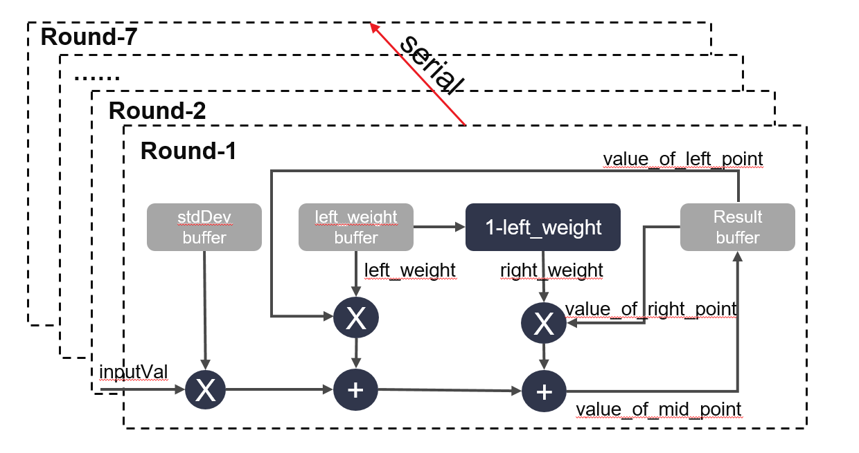
The transform function in class BrownianBridge transform an input sequence with number size to an output sequence. The output data applies to Brownian bridge process. Based on the algorithm, each point in output sequence is generated by previously calculated point. That is to say, each loop dependents on the output of previous loop. To eliminate the loop-carried dependency, we divide the loop into 7 rounds. The loop body only depends on previous round, and the loop in each round has no dependence so that the initiation interval (II) could achieve 1.
The detailed steps of our implementation is as follows:
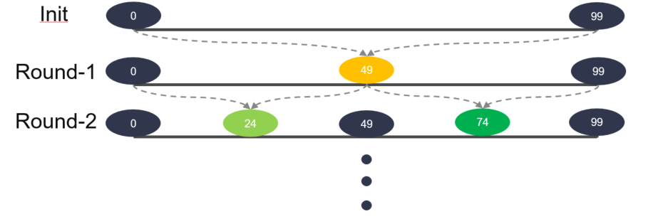
- Init: calculate the value of begin and end point.
- Round-1: divide the sequence into two parts, calculate value of the mid-point. Now the number of sub-sequence is 2.
- Round-2: divide each sub-sequence into two parts, calculate the value of mid-point. Then total number of sub-sequence is 4.
- Round-3: divide each sub-sequence into two parts, calculate the value of mid-point. Then total number of sub-sequence is 8.
- \(\ldots\ldots\)
- Round-6: divide each sub-sequence into two parts, calculate the value of mid-point. Then total number of sub-sequence is 64.
- Round-7: in this round, the distance of each dependency is greater than the loop latency. So the II could achieve 1.
A more discrete description is provided by the following figures. In each round, the order of generated data is from left to right.
Each round shares the same hardware logic named trans_body. It gets begin and end value from the result buffer, then aggregate it with left_weight and right_weight to get the value of mid-point. It is present as follows:
Profiling
The hardware resources for Brownian bridge with sequence length 128:
Engines BRAM DSP Register LUT clock period(ns) Brownian bridge 15 42 16297 10246 3.080
The hardware resources for Brownian bridge with sequence length 1024:
Engines BRAM DSP Register LUT clock period(ns) Brownian bridge 19 33 16219 13056 3.351
The correctness of Brownian bridge generation is verified by comparing results with QuantLib Brownian bridge using the same input sequence. The results are identical.